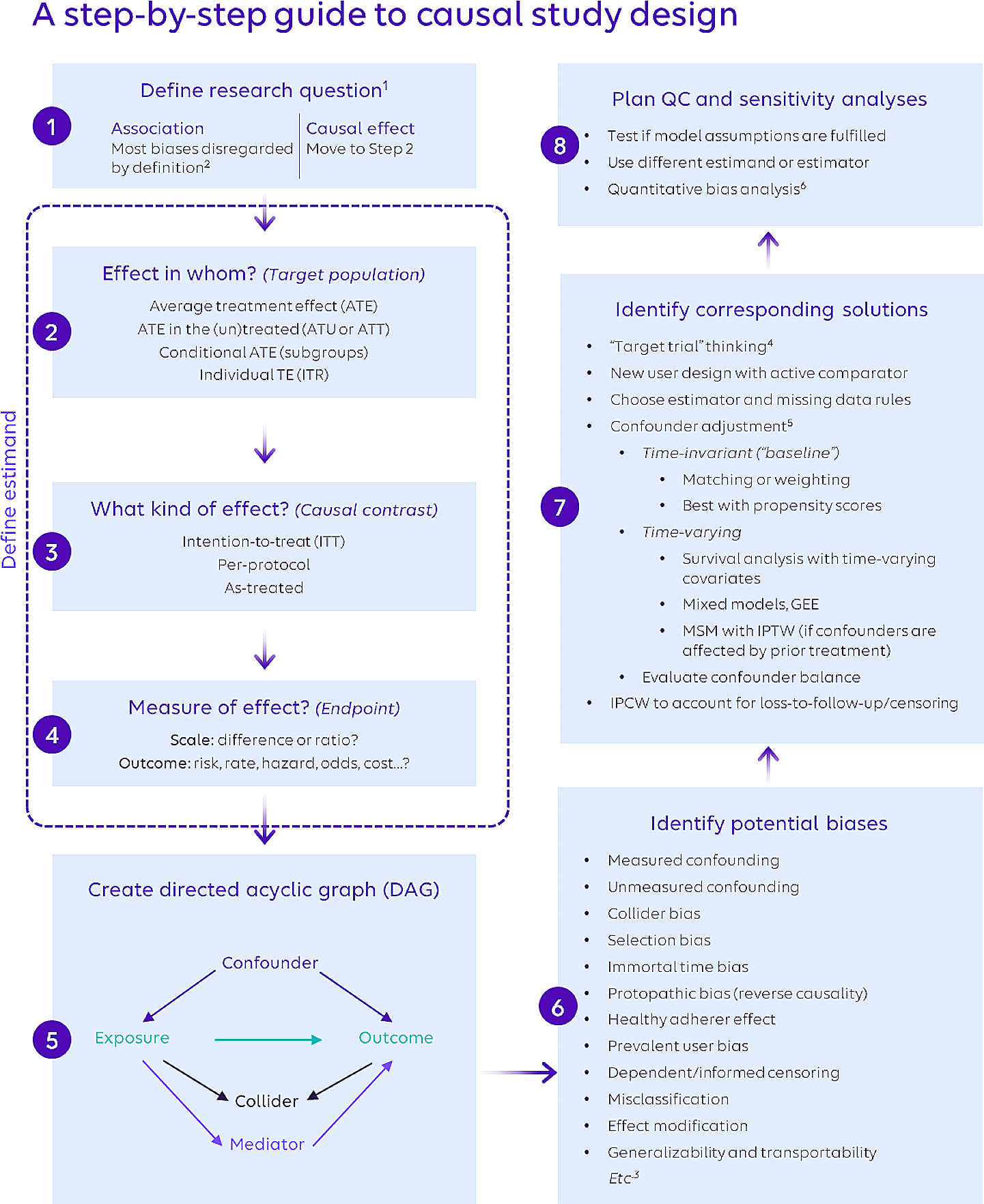
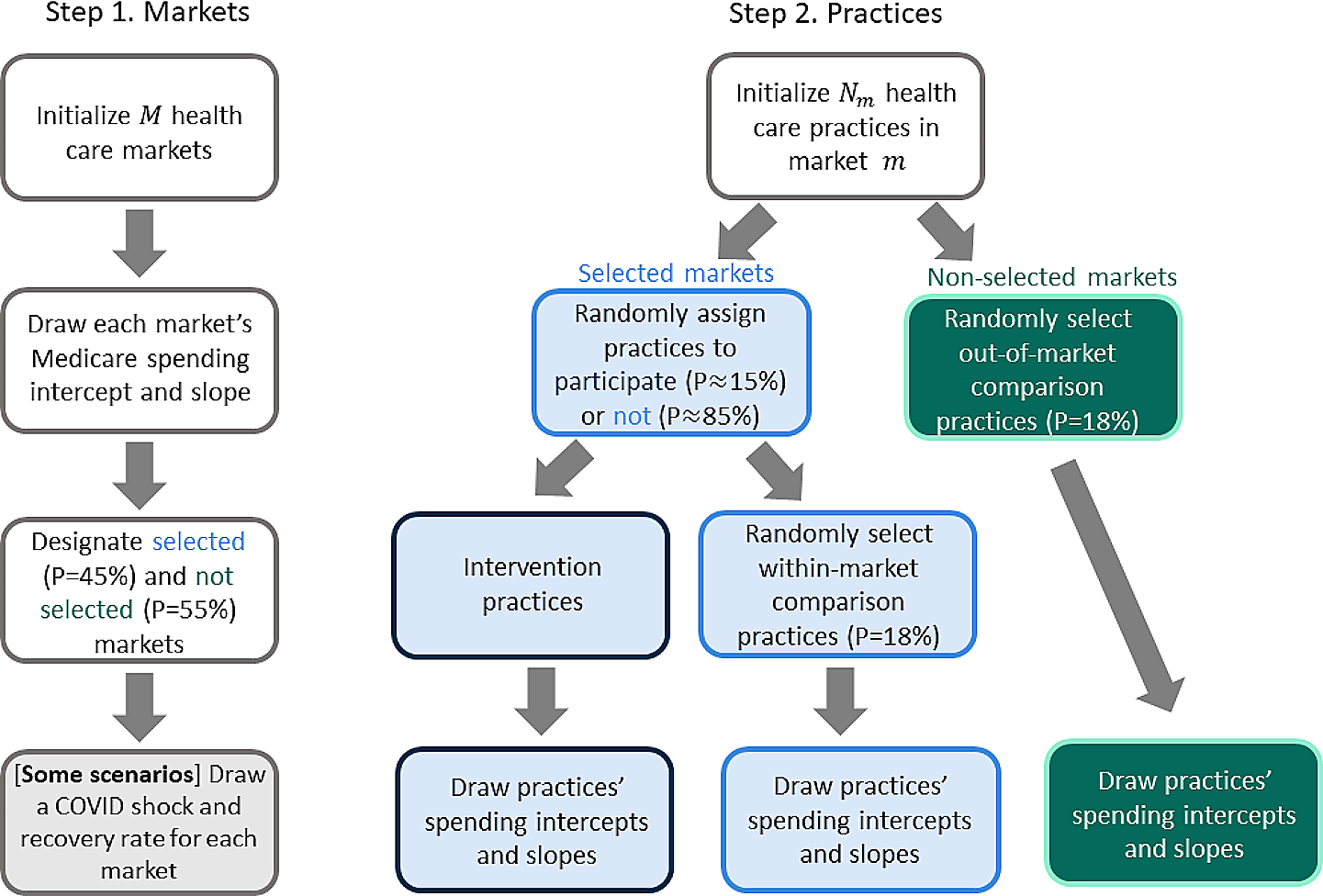
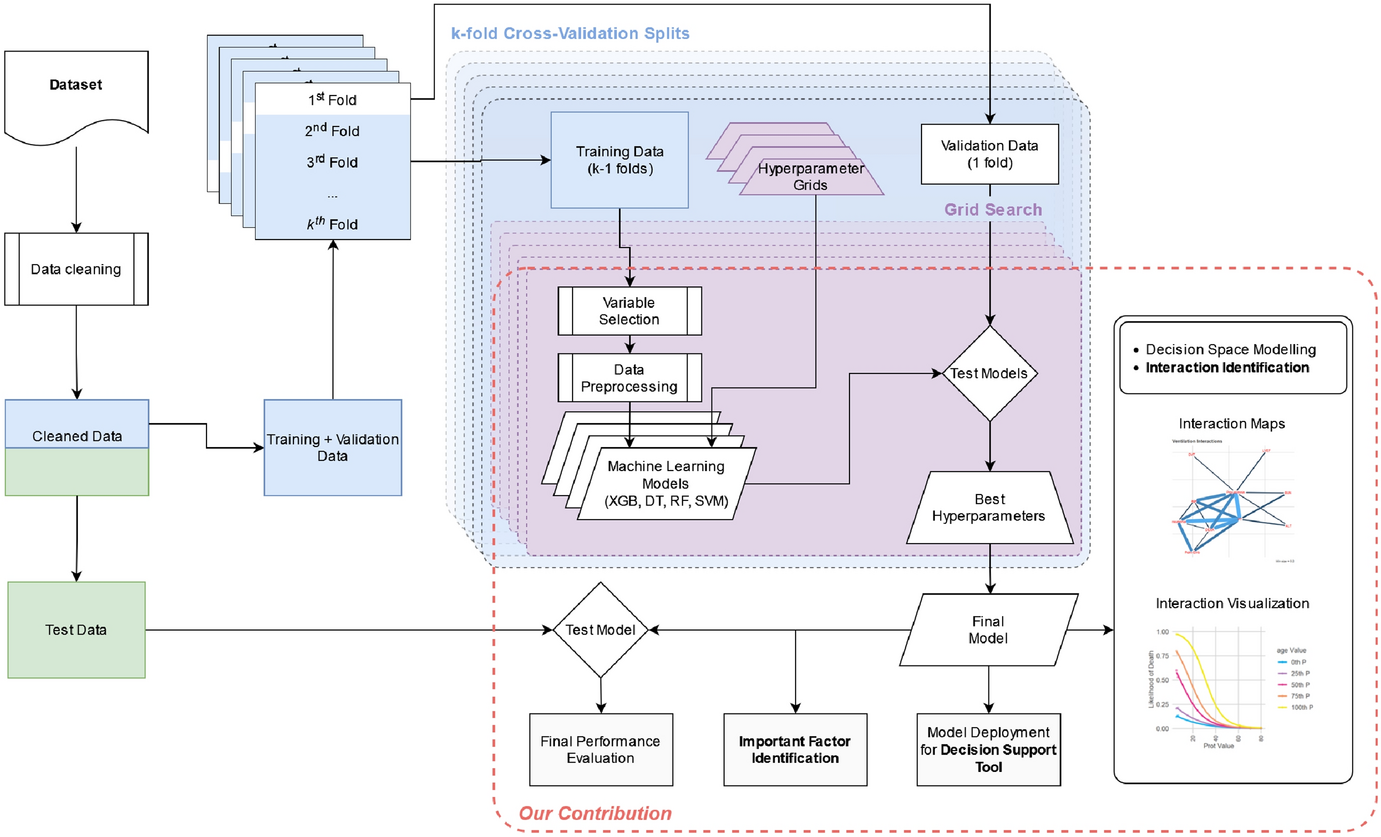
Figure 1 shows the proposed ML framework that enables (1) a methodology that can be used to remove problematic predictors to understand important predictors, (2) a novel exploratory methodology to identify potential interactions between the predictors that can be used to make informed policy decisions, and (3) a unique ML framework that proposes an end-to-end pre-to-post diagnostic testing methodology for COVID-19 that is useful for managers for tactical and strategic decision-making as well as for researchers and domain experts for novel interaction identification that can be used for generating new hypotheses. In the following sections, we describe the various components of this methodological pipeline.

Fig. 1

ML framework for each outcome proposed in this work

3.1 Dataset and preprocessing

The dataset used in this work was released by the VHA Innovation Network in partnership with precision FDA for a competition to invite researchers to model the data in order to further the understanding of the disease (VHA Innovation Ecosystem and precisionFDA COVID-19 Risk Factor Modeling Challenge 2020). To protect patient identity, synthetic health records were generated using Synthea (Walonoski et al. 2018), a well-accepted method to generate research-ready anonymized data. Numerous studies show this method, as well as other synthetic methods, work as well as real data for large population sizes for the purposes of predictive analytics (Benaim et al. 2020; Chen et al. 2019; Gebert et al. 2018; Zhang et al. 2020).

Use of synthetic datasets in the healthcare ML community is common given the many barriers to quality data access (King et al.; Spasic and Nenadic 2020). In this case, the situation is worse given the high potential economic value of such data, thus resulting in complete unavailability of clinical or EHR datasets for COVID-19 patients. The VHA graciously provided this dataset, based on the vast population under their care, and this was made possibly only because of this anonymization.

The dataset consisted of 16 files structured in the standard EHR format, which are listed below. Data dictionaries for these files can be found on the Synthea Github wiki [34].

The dataset contained medical records for 117,959 patients. These records included lab tests, clinical observations, conditions, allergies, patient encounter data and more. It is important to note though that differing amounts of data were available for each patient. The data, as provided, was structured in the long format, i.e., one column lists the name of included variables, while another column lists their corresponding values.

In our study, we processed time-series observations from immunizations, conditions, allergies, and encounters tables by converting them into additional features within our primary analysis table, effectively transforming the dataset into a cross-sectional format. Specifically, for immunizations and conditions, we counted occurrences and used these counts as features, while for allergies and conditions currently affecting the patient at the time of COVID-19 testing, we encoded their presence as binary variables. By doing so, we collapsed the longitudinal data into a single row per patient, enabling the application of ML algorithms that require a fixed number of features for each instance. This conversion was paramount as it allowed us to include temporal clinical events as part of our cross-sectional predictive modeling framework, ensuring that each patient's record reflected their medical history up to the point of COVID-19 testing without directly modeling the data as a time series.

A consequence of this process was that in case a given patient did not have a certain test or encounter in their records, the test would be marked as a missing value in the data. Given the large number of possible tests and encounters included in the dataset, this resulted in a large number of missing values in the dataset as not every patient has had every test and encounter. As such, for this analysis, an ML model that can inherently deal with missing values was used to reduce the complexity of the analysis. Additionally, for the prediagnostic prediction model (i.e., predicting infection), patient data up to the day before the patient presented themselves for a COVID-19 test was used. For postdiagnostic prediction models (i.e., the rest of the models), patient data up to and including but not exceeding the day of COVID-19 testing was used.

Data from selected tables shown above was combined into a single table with each row corresponding to each patient with their corresponding records and outcomes. After preprocessing, the dataset included 492 predictors and five outcome variables. However, the dataset had 63% missing values for the input predictors. These missing values only occurred in columns constructed from tables that had differing levels of information for different patients, i.e., in the observations.csv file, as shown in Table 2. For example, for allergies and conditions, a patient could be labelled to have an active allergy or condition if an active record of one exists. If no record exists in this case, an assumption of no allergy or condition can be made. However, in the case of medical tests, different patients have different medical tests on record, and no assumptions about missing tests can be made outright.

Table 2 File structure of dataset used

Since our dataset had 63% missing values, we used a tree-based models, i.e., extreme gradient boosting (XGB) Chen et al. (2015) and CART decision trees (DT) to model the various outcomes in the data. Furthermore, since support vector machines (SVM) and random forest (RF) do not work with missing values, data for these models was preprocessed to impute missing values with the median value for each variable.

Details about the outcome variables included in the dataset are provided in Table 3. Variable selection and variable importance criteria are detailed in the next section. A file with a complete list of the 492 predictors from the raw dataset (Synthea 2020) and their descriptions can be found in "Appendix B".

Table 3 Outcome descriptions

To ensure that our models provide good predictive performance using factors available at decision-time without future leakage, each of the models is trained based on related EHR data that is available up to a certain date, as shown in the last column of Table 3. For example, for the model prediction infection, the model is only trained and tested using EHR data available up to the day before the patient is presented for covid-19 testing.

3.2 Variable selection and importance

Based on the “splitting” criteria used by tree-based algorithms (refer to Chen, He [35]), one way to find the most important variables in such tree-based algorithm is to look at which variable was used to create the most splits in the learned model. The top 30 most important variables are reported for each outcome in this work.

Given the aforementioned “splitting” criteria used in XGB and other tree-based algorithms, it is important to note that such algorithms use the variables that create the “cleanest” splits for the outcome between the data at each node. Thus, at each split (i.e. node in a tree), the algorithm will randomly choose a subset of variables and within these, it will choose the variable that differentiate the data into the outcomes most efficiently. This highlights the fact that factors included in ML models highlight associations with the outcome only.

Another consequence of the above is that some variables may dominate variable importance in the learned model because it would be used for almost all splits in the algorithm. A very high importance can indicate one of only two things: (1) a very strong predictor (in the case of a simple X → Y mapping), or (2) a problematic variable (in the case where it is unlikely that X → Y is linked so strongly through a single variable). Given that our outcomes are highly complicated problems, it is unlikely that these outcomes can be mostly explained with a single variable. As an example, before variable selection, following were the top variables for each model.

In Table 4, only variables with a variable importance greater than 1% are shown. For the Infected model, three variables cumulatively contribute to 93.95% of the splits in the model. An XGB model trained on just these three variables has an AUC of 0.9811 and a sensitivity and specificity of 99.99% and 96.39% respectively. However, it is unlikely that our outcome can be explained to such an extent using just these three variables. Indeed, this can be confirmed when this simplified model is tested with the holdout set, where its prediction performance (AUC = 0.902, Sensitivity = 69.7%, Specificity = 99.6%) does not match the validation performance, an indication that the model does not generalize. The same principle is true for all the other models as well, as shown in Table 4.

Table 4 Variable importance without problematic variable removal

As such, problematic variables were dropped from the analysis for that outcome since they may be exhibiting simultaneity problems with the outcome or causing the model to overfit on invalid patterns due to missing data. This was done using an iterative model training method:

1.

Start with the complete dataset

2.

Train model using dataset

3.

Observe most important variable

4.

If importance is very high, remove the variable from the dataset

5.

Repeat from 2 until the highest importance variable, either:

a.

Is below a threshold of 0.35 and the next highest importance variable is lower; or

b.

Should remain in the dataset based on expert opinion

The precise cutoff for each model was chosen based on the biggest importance score drop achieved against the smallest AUC or RMSE drop, which also led to a reasonable final AUC. An example of the importance/AUC drop for the death outcome is shown in Table 5. The table shows the most important variable as well as performance metrics for XGB models iteratively trained using the above method. Note that each row signifies a model that was trained without the variables in the rows above it. In the case of this example, it can be seen that the model’s AUC does not change significantly down to the last rows, with row 11 showing the point chosen for the final model. As an example, the model in row 1 uses one variable for 93.9% of its splits, with a handful of other variables used for the remaining splits. As such, if a single factor explained COVID-19 death to such an extent, it would have been widely known by now.

Table 5 Dominating variable behavior against model accuracy

Given computational constraints (model tuning and training with variable selection), the variable selection procedure was performed only with XGB, given XGB is expected to perform the best, and at a fraction of the training time of the remaining models.

3.3 Cross validation and model training

To ensure the validity of ML model, we use a nested cross validation technique as shown in Fig. 2. The larger the test set, the more confident we can be in the performance metrics reported by the model. If the model’s performance metrics for the test set (referred to as the holdout set in this work) are very close to the model’s performance for the training set, it indicates that the model is not over- or under-fitting the data and has correctly generalized the relationships present in the data.

Fig. 2

Nested cross-validated train pipeline

We chose XGB because in applied ML problems, XGB is currently the best performing algorithm across all disciplines as is evidenced by leaderboards across all disciplines as well as its dominance in the academic literature in the past couple of years. XGB is resilient to overfitting (Chen et al. 2015) and can also inherently deal with missing values by imputing missing values at each split that minimize error at that split (Chen et al. 2015). Decision trees (DT) is one of the oldest and simplest learning algorithms, popular for its explainability. It works by splitting the data into segments successively, based on some splitting criteria, creating a tree structure that terminates based on a stopping criteria (Safavian and Landgrebe 1991). Support vector machines (SVM) are a popular kernel based learning algorithm that works on the basis of separating the data based on hyper-planes in a higher-dimensional space than the original data using the “kernel trick” (Osuna et al. 1997). Finally, random-forest (RF) is a widely-used tree-based learning algorithm that uses an ensemble of decision trees that are trained as weak learners in order to minimize over-fitting, a problem that individual decision trees are prone to (Breiman 2001). These remaining models were chosen to serve as a comparison against XGB. These models (DT, SVM and RF) took longer to train (by a factor of 10–1100 compared to XGB) and were therefore not used for our variable selection process. Detailed descriptions of these models are not included in this work, given length constraints. However, the interested reader can refer to (Boulesteix et al. 2012; Noble 2006; Song and Ying 2015) for more information about these models.

Based on preliminary analyses, using more than 30% of the data did not improve performance metrics of the ML models. This was ascertained by splitting the data into chunks of 5% and repeatedly training the ML models with additional chunks until the performance metrics stopped increasing. Therefore, for this work, 35% of the data was used for training and parameter tuning with fivefold cross-validation (Fushiki 2011), while the remaining 65% was used as the holdout set.

All ML models produce numeric outputs, both for classification or regression problems. For binary classification problems, ML models produce a continuous number between a range, usually 0–1, to signify a binary outcome, which is produced by comparing the continuous output against a threshold. A general starting point is to use 0.5 as a threshold; however, choosing 0.5 may lead to lower prediction performance in some metrics. As such, this threshold can be selected based on the receiver operator characteristic area under the curve (AUC) graph, to choose a point for best balance between accuracy for both classes (i.e., points closest to the top left corner of the graph), or to favor accuracy for either class, based on the requirements of a given problem. This type of threshold selection is called post-hoc threshold selection. In this work, we use post-hoc threshold selection for the classification models. The validity of each threshold is confirmed with the hold-out set.

Model parameters were tuned with a grid-search methodology to find the parameters that resulted in the best model performance. All tuning was done using fivefold cross-validation. Additionally, as can be seen in Table 1, the Death and Ventilation outcomes were severely imbalanced in the dataset. In our preliminary experiments, the model performance unfortunately did not improve with any synthetic generation algorithms like SMOTE (Chawla et al. 2002). The post-hoc threshold selection (Zhao 2008) was sufficient to provide a model that had balanced sensitivity vs. specificity, which was confirmed with the cross validation and subsequently the holdout sets.

3.4 Performance metrics

Since we have both classification and regression models in this work, we report the AUC for the classification models and the RMSE (root-mean-squared error), R2 and MAPE (mean average percentage error) for the regression models. The AUC is chosen for the classification models since it shows the models performance at all possible decision thresholds (i.e., all sensitivity/specificity pairs), however we also report the best sensitivity/specificity pair. The best pair from the holdout set is calculated based on threshold selection from the training set. Formulae for each of these measures are given below and Davis and Goadrich (2006) provide detailed explanations.

$$Sensitivity=\frac$$

(1)

$$Specificity=\frac$$

(2)

$$MAE=\frac^\left|_-_\right|}}}$$

(5)

3.5 Interaction effects

Using a novel methodology (Nasir et al. 2021), the top 30 variables for each outcome’s model are also examined for possible interaction effects with other variables present in each respective model based on the best performing ML models, i.e., XGB, for each outcome. Since the ML models are non-parametric, it is impossible to directly see how the models make predictions (Guo et al. 2021). However, given the models are making good predictions based on the relationships they learnt from the training data, these relationships can reveal information about the phenomenon described by the data.

To find these relationships, we perform sensitivity analysis for all predictor pairs that include the top 30 important variables, which allows us to observe if and how one variable impacts the effect of another variable on a given outcome. This is done by changing this variable pair’s values while keeping all the other variables fixed at their means, while observing the output. Variable pairs that demonstrate an interaction are detected using this methodology. Variables that are observed to have a large effect on the outcome as well as an effect on the effects of other variables can be deemed to be highly important for the outcome. The detailed algorithm for this methodology is provided below.

1.

Start with a dataset where a mapping between inputs (X’s) and an output (Y) exists.

2.

Model this mapping using one or more ML models. We use five XGB models, each trained using four alternating folds out of five from the training dataset.

3.

For each variable pair:

3.1

Split the input domain into quintiles.

3.2

With each model:

3.2.1

Plug in each variable combination to map the variable pair’s behavior.

3.2.2

Subtract the quintile mean from each quintile (line).

3.2.3

Sum up the area between the resulting curves to get the effect “size”.

3.3

With all the models’ resulting effect sizes, calculate the mean, standard deviation and coefficient of variation (CV) of the size.

4.

Filter variable pairs based on mean and CV values, selecting variable pairs with large mean and small CV values.