Patient

YL is a right-handed male in his late twenties. He underwent an operation for a left hemispheric, low-grade intraventricular tumour and developed a dense right homonymous hemianopia after surgery, three years prior to this study. Subsequent clinical testing revealed signs of residual visual motion perception in his blind (right) hemifield. He was referred to our study via a specialist outpatient visual service run at the National Hospital for Neurology and Neurosurgery in London. He gave informed written consent to participate in our study, which had been approved by the Yorkshire and the Humber—South Yorkshire Research Ethics Committee (NHS Health Research Authority) and UCLH/UCL Joint Research Office (protocol number 137605).

Experiment 1

The aim of this experiment was to establish whether YL could consciously perceive visual motion in his blind field, and to determine his neural responses while doing so. We assessed the former with psychophysics and the latter with fMRI.

Psychophysical testing

We used achromatic random checkerboards (40% contrast) that were either static or drifted upward or downward at a speed of 20°/s (Fig. S1). The stimuli subtended 12° in width and 22° in height and were confined to YL’s blind (right) field, 6° to the right of the vertical meridian. During the psychophysics session, YL was asked to indicate the motion direction of the stimulus after each presentation, following a two alternative forced choice (2AFC) approach, and to indicate his certainty of the response on a three-point scale, one indicating “complete guess”, two “I think I saw motion, but I’m not sure of its direction”, and three “I definitely saw the stimulus moving up (or down)”.

MRI data acquisition and procedure

Based on the results of the psychophysics studies, YL underwent MRI scanning at the Wellcome Centre for Human Neuroimaging. We collected data on a 3 T Siemens Magnetom Prisma scanner (Siemens Healthcare GmbH, Erlangen, Germany) including structural, volumetric T1w images to assess the extent of his lesion, fMRI data to assess his neural responses to visual motion, and multishell diffusion MRI to perform a tractographic reconstruction of his optic radiations.

Structural imaging was based on the 3D magnetisation-prepared accelerated gradient echo (MPRAGE) sequence: repetition time (TR) = 2.53 ms; echo time (TE) = 3.34 ms; flip angle = 7°; matrix of 256 × 256; field of view = 256 mm; voxel size = 1 × 1 × 1 mm3.

To assess visual motion responses, we collected data from two fMRI runs during which we presented YL with the same random checkerboard stimulus (Fig. S1), either statically or in motion (20°/s), as well as a ‘blank’ condition during which no stimulus was shown. Each of the three conditions was presented eight times in blocks of approximately 20 s. To ensure that YL was fixating the screen’s centre, he engaged in a fixation task by pressing a button in response to a brief (300 ms) colour change in the fixation cross that occurred at random throughout the acquisition.

fMRI data was based on the blood oxygen level dependent (BOLD) signal, measured with a 2D T2*-weighted echo planar imaging (EPI) sequence: volume TR = 3360 ms; TE = 30 ms; flip angle = 90°; ascending acquisition; matrix of 64 × 64; voxel size = 3 × 3 × 3 mm3; 48 slices. Two fMRI runs were acquired. Field mapping images were also acquired using a dual-echo gradient echo sequence to assist with susceptibility distortion correction.

Diffusion MRI data was based on a 2D spin-echo EPI sequence: TR = 3500 ms; TE = 61 ms; flip angle = 88°; matrix of 110 × 110; voxel size = 2 × 2 × 2 mm3; 72 slices; multiband factor of 2; in-plane acceleration factor of 2. Images were acquired with four diffusion shells: 30 diffusion directions at b = 500 s∙mm−2, 60 directions at b = 1500 s∙mm−2, 90 directions at b = 2500 s∙mm−2, and 120 directions at b = 6000 s∙mm−2. In addition, 25 b = 0 s∙mm−2 were interleaved throughout the acquisition, and seven b = 0 s∙mm−2 volumes were acquired with the reverse phase encoding polarity to correct for susceptibility distortions.

MRI data pre-processing and analysis

The T1w image was skull-stripped using optiBET (Lutkenhoff et al. 2014), bias field corrected using the N4 tool (Tustison et al. 2010), and rigidly aligned, using flirt (Jenkinson et al. 2002), to the 1 mm MNI T1w brain template as a substitute for AC-PC alignment. This aligned image served as the anatomical reference for subsequent pre-processing and analysis steps.

The first four volumes of each fMRI run were discarded to allow the scanner to reach steady state. The remaining images were corrected for motion and slice-timing differences using SPM12 (http://www.fil.ion.ucl.ac.uk/spm/software/). The corrected images were then simultaneously corrected for geometric distortions (based on the acquired field map) and aligned to the T1w image using FSL’s epireg tool (Greve and Fischl 2009; Jenkinson et al. 2002), while maintaining the voxel size at 3 × 3 × 3 mm3. The BOLD time series images were then spatially smoothed with a Gaussian kernel of a full width at half maximum (FWHM) of 4.5 mm. This produced the final fMRI time series images that were used in subsequent analyses.

A standard GLM was fit to the time series, with a task effect (stimulus presentation) for each of the moving and static conditions, and six motion correction parameters as nuisance regressors. Categorical comparisons were performed to identify the brain regions in which activity increased in response to the presentation of the moving and static random checkerboards. All resulting statistical images were thresholded at a voxelwise significance level of p < 0.001. This was done in SPM12.

Raw DWI data was first corrected for noise and Gibbs ringing artefacts (Kellner et al. 2016; Veraart et al. 2016). A magnetic susceptibility field was then calculated using topup (Andersson et al. 2003) based on b = 0 s∙mm−2 images acquired with opposite phase encoding. All images were subsequently corrected for motion and eddy current distortions using eddy (Andersson and Sotiropoulos 2016) with outlier (signal dropout) slice replacement (Andersson et al. 2016), incorporating the topup field into this step. The anisotropic power map was derived from the pre-processed data using StarTrack (www.mr-startrack.com) and used to calculate a rigid affine transformation (six degrees of freedom) to the T1w image with flirt (Jenkinson et al. 2002). The rigid transformation was then applied to the diffusion data (kept at a 2 mm voxel size) with a spline interpolation to produce the final set of pre-processed images. The diffusion gradients were also rotated at this stage using the same transformation matrix.

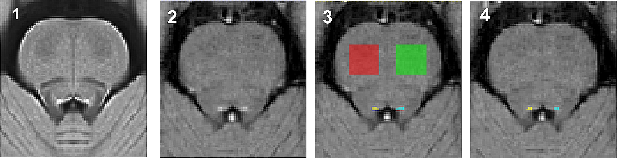
The diffusion data was used to reconstruct the optic radiations connecting YL’s lateral geniculate nucleus (LGN) to his visual cortex. The data from the two highest shells (b = 2500 and 6000 s∙mm−2) were modelled with spherical deconvolution based on the damped Richardson-Lucy algorithm (Dell’Acqua et al. 2010, 2013) in StarTrack, according to the following parameters: fibre response α = 1.5; number of iterations = 200; amplitude threshold η = 0.001; geometric regularisation ν = 16. A probabilistic dispersion tractography approach was followed to explore the full profile of the fibre orientation distribution function (fODF) in each voxel according to the following parameters: minimum HMOA threshold = 0.001; number of seeds per voxel = 2000; maximum angle threshold = 45°; minimum fibre length = 35 mm; maximum fibre length = 200 mm. This was done using a manually defined seed region of interest in the LGN. The resulting tractogram was imported into TrackVis (http://trackvis.org/) where manual cleaning was performed and streamlines terminating in visual cortex were selected. The final dissected white matter tracts were divided into 100 equidistant segments and microstructural mean and standard deviation metrics were calculated for each.

Experiment 2

The first experiment revealed that YL can perceive motion in his blind field consciously, that his visual cortex is responsive to moving but not static visual stimuli, and that his optic radiations, though damaged, still connect his visual cortex with the thalamus. This led us to hypothesise that the M and P systems are differentially affected in his brain; we therefore conducted additional experiments to address this question.

Psychophysical testing

We used achromatic sine wave checkerboards (Fig. S2) that varied in spatial frequency (0.3 or 1.4 cycles/°), contrast (20% or 80%), and speed (1 or 8°/s). We collected a total of 224 trials over seven task runs, which included 28 trials per condition. YL was asked to give his response and his certainty to the perceived direction of motion as in Experiment 1. The stimuli were confined to the same location in his blind field.

MRI data acquisition and procedure

Based on the psychophysics results, YL underwent further MRI scanning at the Wellcome Centre for Human Neuroimaging; we collected data on a 7 T Siemens Magnetom Terra scanner including structural, volumetric T1w images, and fMRI data.

A T1w volume was acquired based on a 3D fast low-angle shot (FLASH) sequence with the following parameters: TR = 19.5 ms; TE = 2.3 ms; flip angle = 24°; field of view = 364 × 426 × 288 mm3; voxel size = 0.6 × 0.6 × 0.6 mm3.

We collected two fMRI runs during which we presented YL with P- and M-type stimuli, as well as blank trials. The P stimulus was a sine wave checkerboard with a spatial frequency of 1.4 cycles/°, 90% contrast, and drifting at a speed of 1.5°/s (Figure S3). The M stimulus had a spatial frequency of 0.35 cycles/°, 30% contrast, and a speed of 16°/s (Fig. S3). Each stimulus was presented eight times in blocks of approximately 24 s, interleaved by blank blocks of approximately 12 s. The stimulus subtended 20° in width and 10° in height due to the limited screen size at 7 T, simultaneously targeting both hemifields, and was masked with a grey disk (3° in diameter) in the centre to ensure that the fixation cross remained visible. Here, again, YL engaged in a fixation task.

The BOLD signal was measured with a 3D T2*-weighted EPI sequence: volume acquisition time = 2332 ms; TR = 53 ms; TE = 20 ms; flip angle = 15°; field of view = 192 × 192 × 88 mm3; voxel size = 1 × 1 × 1 mm3; PAT acceleration factor of 8; partial Fourier 6/8 in the phase-encoding direction. Four additional EPI volumes were acquired with the opposite phase encoding to be used later for distortion correction.

The main differences between psychophysics and fMRI in the second experiment were (1) the speed of the M stimulus and (2) the stimulated field of view. Regarding the first point, we chose a higher speed for the M stimulus during fMRI to ensure that BOLD signal changes to motion stimuli were strong enough and distinguishable enough from the slow stimulus. As for the second point, we only stimulated the blind field in psychophysics to ensure that the patient was not aware of the stimulus properties (e.g., texture or contents) during the direction discrimination task, while during fMRI we stimulated both hemifields simultaneously to include as many blocks of the localiser task as possible after having established the behavioural responses offline.

MRI data pre-processing and analysis

The T1w image was aligned with the structural image from the 3 T session for ease of comparison and served as the reference for the 7 T fMRI pre-processing steps. This was achieved through a rigid-body alignment performed using flirt (Jenkinson et al. 2002).

The fMRI images were first denoised using NORDIC (Vizioli et al. 2021). Then, the first two volumes of the first run were combined with their opposite phase-encoding counterparts and passed to topup to calculate the susceptibility distortion field (Andersson et al. 2003). Afterwards, the images from both fMRI runs were concatenated and passed to eddy (Andersson and Sotiropoulos 2016) where motion correction and susceptibility distortion correction (based on the topup field) were simultaneously applied, accounting for the effect of motion on these distortions (Andersson et al. 2018). The corrected images from both task runs, all of which were in alignment at this stage, were then aligned to the structural T1w image by way of a rigid-body alignment performed in flirt (Jenkinson et al. 2002) using the mutual information cost function and spline interpolation. Finally, the images were spatially smoothed with a Gaussian kernel of a FWHM of 1.0 mm.

The first four volumes of the time series were discarded, and a standard GLM was fit to the data with a task effect (stimulus presentation) for each of the M- and P-type conditions, and six motion correction parameters as nuisance regressors. Categorical comparisons (t test) were performed to identify the brain regions in which activity increased in response to the presentation of each type of stimulus relative to a grey background; additionally, the two conditions were directly compared with each other. All resulting statistical images were thresholded at a voxelwise significance level of p < 0.001. This was done in SPM12.

Statistical analysisPerformance

We calculated YL’s accuracy on the motion direction discrimination task as the percentage of correct trials. For instance, for a given condition (e.g., low frequency, high speed, high contrast), accuracy, A, was calculated as:

$$A=\frac_}_+_}\times 100$$

(1)

Given that the direction response had two possible outcomes only with equal probability (50% each), we used the binomial distribution based on the appropriate number of responses (trials) to determine whether accuracy was significantly above chance for a given task condition. We performed these analyses using the binocdf function in MATLAB (The MathWorks).

Certainty

To ease the interpretation of the certainty scores, which were collected on a three-point scale, we converted each trial’s certainty score to a percentage value as follows:

$$_=\frac\times 100$$

(2)

where C is the original score obtained on the three-point scale (values between 1 and 3), and Cperc is the certainty score in percentage terms. Therefore, Cperc = 0% would indicate the lowest certainty possible (i.e., complete guess), Cperc = 50% would indicate moderate certainty, and Cperc = 100% would indicate the highest level of certainty.

Certainty vs. accuracy

To assess whether YL’s certainty for each condition was related to his accuracy, we used Pearson’s correlation with one-tailed significance testing. We did this to test the direct relationship between mean certainty and accuracy for the eight conditions, and to test the correlation between the observed data and the data predicted by the psychophysical model proposed by Zeki and ffytche (1998).

Effect of stimulus properties

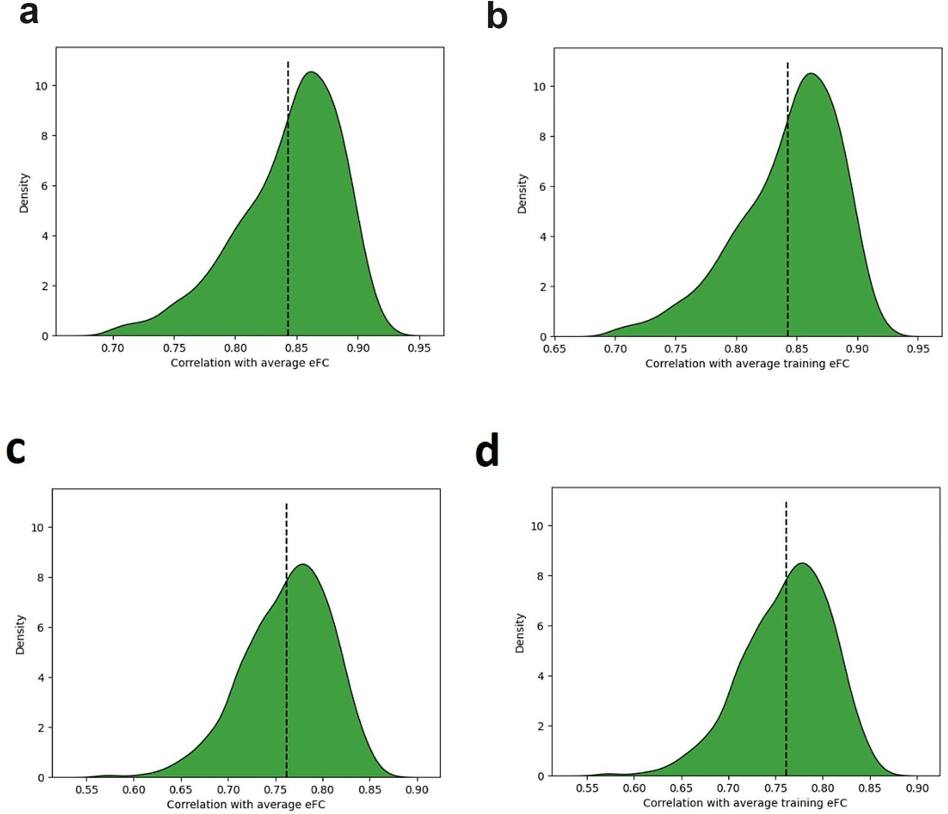
We further tested YL’s responses to assess the effect of spatial frequency, contrast, and speed on his performance. We trained a linear model, using maximum likelihood estimation, on 75% of the non-blank trials (N = 158) to predict whether YL’s response to a given combination of spatial frequency, contrast, and speed would be correct using frequency as the only predictor (Model 1). We then trained a second model using all three factors as predictors (Model 2). We then applied the same approach and trained two linear models to predict YL’s certainty using frequency as a sole predictor (Model 3) or using all three factors as predictors (Model 4). We tested each model’s predictions on the remaining 25% of trials (N = 53) to assess whether it generalises well to the rest of YL’s responses. We also applied the likelihood ratio test to assess whether including speed and contrast improved each model’s predictive power.