We used unit data from the fifth round of the National Family Health Survey (NFHS) conducted between 2019 and 2021. NFHS is a large-scale multi-round survey providing comprehensive information on population, health, and nutrition across India and each state/union territory (UT). The recent round, i.e., NFHS-5, covered newer topics, such as preschool education, disability, access to a toilet facility, death registration, bathing practices during menstruation, and methods and reasons for abortion. The survey successfully interviewed 2,843,917 household members from 636,699 households, among which 724,115 women aged 15–49 years and 101,839 men aged 15–54 years, along with other age group people, using a multistage stratified sampling design. Detailed information on study design, sample, collection, and available findings are in the national report [35]. This study is based on secondary data available in the public domain; written informed consent was obtained from all participants during the survey. Therefore, there was no need to obtain ethical clearance for this study.

The final analytical sample included 27,93,971 individuals from 636,189 households nested within 30,170 clusters, 707 districts, and 36 states/union territories (Additional file 1: Figure S1). The final selection includes only the de jure population and excludes those having missing covariates. Additional file 1: Table S2 extensively provides the number of districts, clusters, total individuals, and disabled individuals nested within each of the 36 states/union territories. Uttar Pradesh, followed by Bihar, was the largest state with 75 and 38 districts, respectively. Among the individuals, 26,394 had some form of disability, further identified by their disability types.

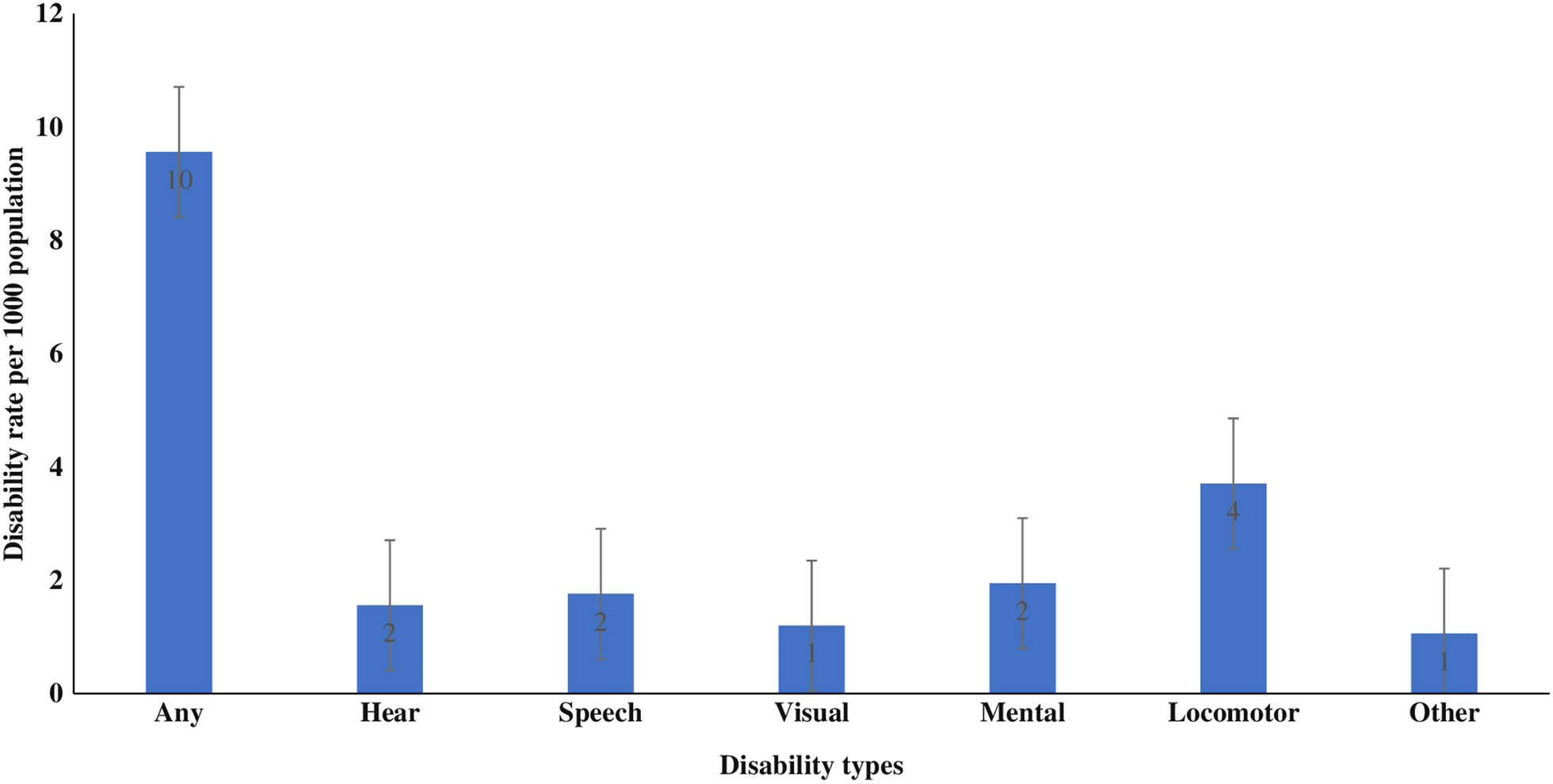
The primary outcome variable was any form of disability. Those with any disability were categorized according to their disability type: hearing, speech, visual, mental, locomotor, and other.

NFHS-5 collected information on the disability status of individuals in the household questionnaire from the de-jure population using the following questions: “Does any usual resident of your household, including you, have any disability?”. The individual was identified with the line number in the household answering “yes,” which was further identified according to their disability types. The description of all kinds of disabilities is provided in Additional file 1: Table S3.

Socioeconomic status is shown through the relative poverty measure, i.e., wealth index [31]. The wealth index is constructed using principal component analysis (PCA) conducted on a set of 37 variables based on household amenities, assets, and consumer durables [36]. The wealth scores generated from the PCA are split into quintiles ranging from the poorest to the richest, with 20 percentiles each. The lowest 20 percent of households were coded as poorest and the highest 20 percent as richest. This was termed the wealth quintile in the analysis and was available in the dataset. The wealth index was computed separately for urban and rural areas.

Based on the prior literature, we included individual, demographic, and household variables as possible confounders [12, 14, 16, 21, 30]. Age is categorised as 0–9 years, 10–19 years, 20–29 years, 30–39 years, 40–49 years, 50–59 years, and 60 + years. Sex as male or female. Education of individuals categorised as no education, less than 5 years, 5–9 years, and 10 + years. Religions as Hindu, Muslim, Christian, and Others. Caste is classified as [Scheduled Caste/Scheduled Tribes] (SC/ST), [Other Backward Caste] (OBC) and Others. The residence is categorised into either rural or urban.

Taking cue from previous literature [37, 38], we included two standard cluster variables by aggregating the individual’s educational level and wealth status: (a) Education level of the cluster, defined as the proportion of individuals with more than 10 years of schooling among all individuals in the cluster. (b) Wealth status of cluster; is defined as the proportion of the rich and richest households among all the households in the cluster. We categorised the proportions of education level and wealth status of the cluster as low, medium, and high. It denotes that the higher the proportion of educated individuals, the higher the cluster’s educational standard. And the higher proportion of rich and richest households means higher wealth status in the cluster.

Similarly, we included two standard variables for districts and states, aggregating the educational level and wealth status. The variables are the Education level of district (low, medium, high), Wealth status of district (low, medium, high), Education level of state (low, medium, high), Wealth status of state (low, medium, high).

Frequency and percentage distributions were used to show participant characteristics. Age -sex-adjusted disability rates (per 1000 population) were reported across the participant characteristics and states. All the analyses and figures presented were prepared in STATA software, and the “syvset” command was used in the study for accounting sampling weights, clustering, and stratification. To assess the socioeconomic inequality in the prevalence of disability (by its type), we measured the Erreygers Concentration Index (EI). It should be noted that the concentration indices are the popular choice of measuring socioeconomic-related health inequality, preferred over relative index and slope index of inequality [39]. The disproportionality-based relative measure of inequality (i.e., Relative Concentration Index, CI) is used to express inequality as a function of shares of the health indicator compared to shares of the population [40].

We used the CI as follows: \(}= \frac cov(_, _)\)

where \(_\) is an indicator of disability type for individual i, \(_\) is the fractional ranking of individuals according to the wealth index, and \(\mu\) is the mean of \(_\) [41].

However, when the outcome variable is a binary indicator, the range of CI often shortens. So, for a more robust result, we have used Erreygers Concentration Index (EI) to address such a problem [42]. It is a normalized form of CI defined as

Here, \(\mu\) is the mean of the disability variable by its type, \(CI\) is the standard CI, b is the maximum value of the disability variable (i.e., 1), and a is the minimum value of the disability variable (i.e., 0).

EI varies between −1 and + 1, with a negative value suggesting a concentration of disability among the poorest and a positive value indicating a concentration of disability among the richest.

Besides wealth, education is also a strong determinant of health, as educated people are more likely to use information effectively and efficiently, making them aware of their health and likely to follow medical advice [43]. So, we carried out sensitivity analyses in which the education of 18 + age individuals were also used to elucidate socioeconomic variations of disabilities. It should be noted that the educational variations were confined to 18 + adults as those in 0–17 years of age are mostly a dependent population who may or may not be responsible for their health decisions. Further, age-sex-adjusted estimates were calculated for disability rates in all inequality dimensions.

The present study used a visual way to illustrate the concentration index through the concentration curve. The concentration curve plots the cumulative percentage of disability variable (by type) on its y-axis against the cumulative percentage of household wealth index/individual education level on the x-axis. If the concentration curve lies above the line of perfect equality, the disability is concentrated among poor/uneducated people, and vice versa [44].

Multivariable analysis using a four-level random intercept logit model showed the risk factors associated with disability across its type, adjusting for all covariates (reporting coefficients with 95% confidence intervals). We adopted multilevel analysis to partition the total geographic variations for the probability of an individual i (level-1) in cluster j (level-2), district k (level-3) and state/UT l (level-4) having a disability (Y) using the equation:

$$}\left( \, = \,1X} \right)} \right)\, = \,_ \, + \,_}}} \, + \,\left( _ \, + \,}_ \, + \,f_ } \right)$$

where the dependent variable Y (disability by its type) and set of independent covariates X were assumed to follow a four-level data structure. \(_\) represents the constant and \(_,}}__\) are residuals specific to cluster, district and state/UT, respectively. The residuals are assumed to be normally distributed with a mean of 0 and variances of \(^}_\), \(^}_}0}\) and \(^}_}0}\). These variances estimate were between clusters within a district (\(^}_\)), between districts within a state/UT (\(^}_}0}\)) and between states/UT within the country (\(^}_}0}\)), respectively. We assumed a fixed individual-level variance of \(\frac^}\) or 3.29 due to binary nature of outcomes [45, 46]. The multilevel model was applied using MLwiN 3.05 software program via the “runmlwin” command in STATA 16.0 with default prior distributions of iterated generalized least square (IGLS) estimation method [47].

It should be noted that the two model specifications, namely the null model (without any covariates) and the adjusted model (controls all the covariates), were estimated based on the above modelling structure. We computed the variance partitioning coefficient (VPC) to assess the significance of each geographical unit in total variability for null and adjusted models, such as for unit z, VPC% = \(\frac^}_}}}^}_+^}_}0}+^}_}0}+\frac^}} * 100\). Further, we carried out a sensitivity analysis using two-level model structures in which individuals were assumed to be nested within only one geographic level. This helps to evaluate the changes in the variance estimates and the proportion of variance attributable to high levels from all four levels to only one geographic level at a time.

Next, we generated district-specific precision-weighted estimates for each type of disability. The probability of disability for each district was calculated as equation: \(\frac}(_+}}_+ _)}}(_+}}_+ _)}\). The precision-weighted probability was further multiplied by 1000 for interpretation clarity. We also generated precision-weighted estimates specific to each cluster for disabilities, calculated as\(\frac}(_+\upmu }_ +}}_+ _)}}(_+\upmu }_ +}}_+ _)}\). The within-district or between-cluster small area variations were computed as standard deviations (SDs) of these estimates. The district-level maps were prepared using QGIS 3.28 software. The shapefile was obtained from the DHS Spatial repository (https://spatialdata.dhsprogram.com/boundaries).