Molecular characterization

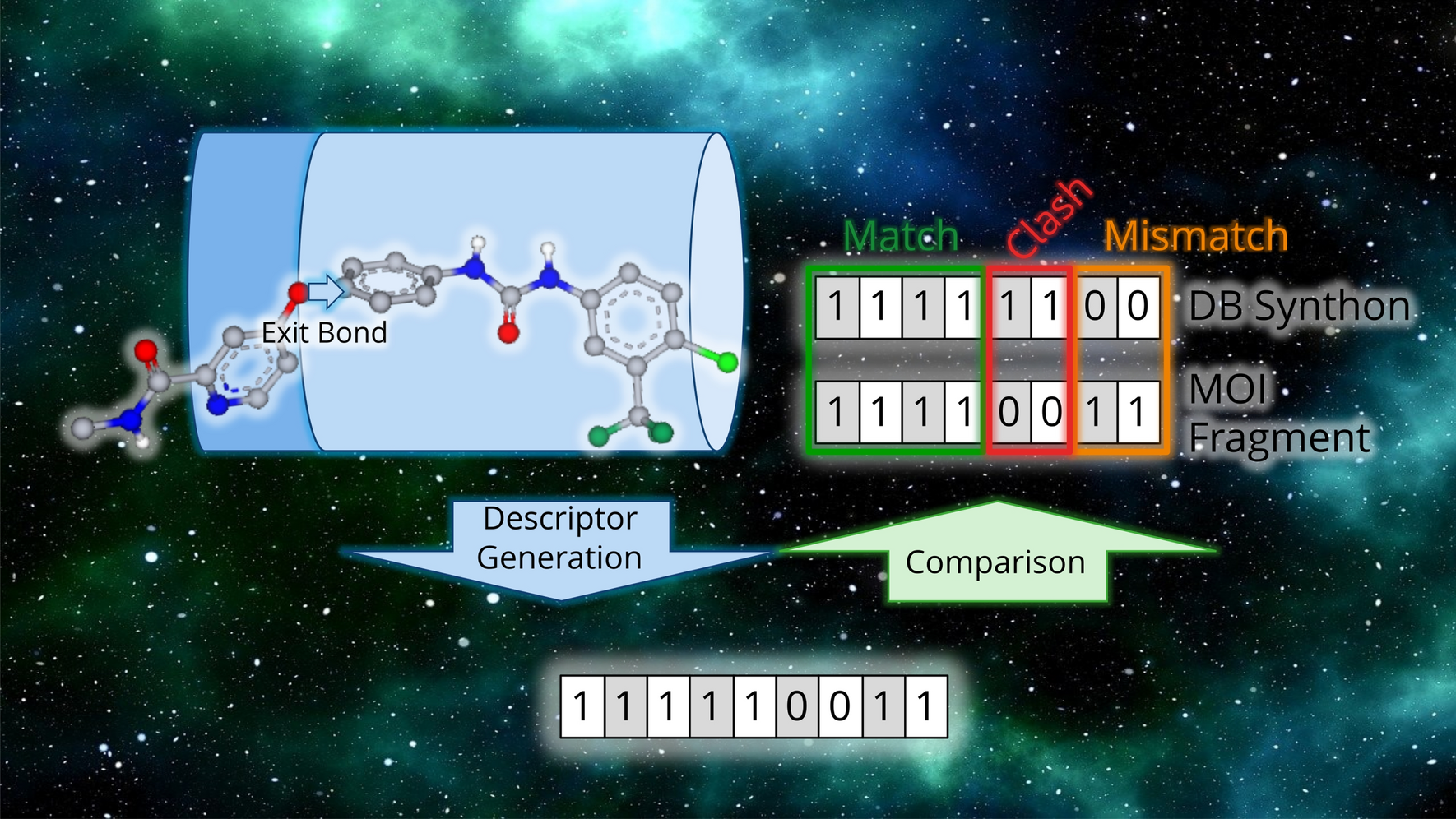
To identify if a molecule is foreign, and if so, what parts are foreign, we defined some simple localized molecular descriptors. Atoms were characterized with atom keys. Atom keys are integer tuples comprising an atom’s degree (D) (i.e. its number of adjacent atoms), valence (V), atomic number (Z), formal charge (Q) and number of hydrogens (H). These properties were chosen because they are largely independent from the atom’s surrounding chemical environment. To avoid cyclic dependencies between properties, in this work valence is defined as the sum of an atom’s bonds’ orders, without considering the atom’s formal charge. The order of the atom key’s properties is relevant. We ordered the properties by perceived decreasing significance or importance. For example, we assume that a change in degree, and therefore topology, is more disruptive to a molecule’s structure and properties than a change in atomic number. Bonds were characterized as a tuple of the bonded atoms’ keys (AK) and an integer representing the bond’s type (B), which can be thought of as the bond’s order (Fig. 2).

Fig. 2

Partial atom and bond key pyramid. Higher order keys encompass lower order keys. The (D, V, Z, Q, H) key constitutes the atom key AK, and (AK1, AK2, B) constitutes the bond key

We also defined partial keys of the atom and bond keys. Partial atom keys were constructed by taking the first j most significant properties of the atom key, with j∈  [1, k-1], where k is the number of properties in an atom key. Consequently, partial key j contains all partial keys with a lower j. The same procedure was applied to bond keys but with the range j ∈ [2, k-1]. This yields a total of four partial atom keys and one partial bond key (Fig. 2). Partial keys can be sorted lexicographically, enabling fast key-value store searches.

Lastly, circular atomic environments were defined for all atoms in the molecules. A circular atomic environment comprises a central atom and all surrounding atoms within a given topological distance termed the environment’s radius r. The resulting atomic environment was hashed to an integer using the Morgan algorithm [33, 34], and said hash was taken as the environment key or unique identifier of the environment. As such, these identifiers are conceptually equivalent to ECFP fingerprint features [34]. The Morgan algorithm requires initial atom identifiers or “invariants”. There is some flexibility in the selection of atomic invariants. By default we use the atom keys’ hashes as invariants, mimicking the Daylight atomic invariants [35]. However one could incorporate other information such as ring membership [34, 36].

Reference dictionary

In this work a subset of ChEMBL31 [10] was chosen as the reference library of drug-like molecules. Only small organic molecules were retained. Large biomolecules, natural products and polymers were excluded. For the remaining molecules the unsalted and non-ionized “parent form” was chosen. Molecules in the reference library were characterized using the aforementioned descriptor keys, and the frequency of each key recorded in a “chemical dictionary”. We generated two dictionaries using environment radii of 1 and 2 respectively. If a key’s frequency surpasses a user-specified threshold (by default 0) it is deemed familiar, and otherwise it is deemed foreign. Owing to the way in which keys are defined, simpler keys are contained by more complex keys. For example, environment keys contain bond keys and bond keys contain atom keys (Fig. 2). This defines unidirectional dependency relationships between them, meaning that if a key is foreign all dependent keys containing it must also be foreign. The reverse is not necessarily true.

Tree search algorithm

The molecule correction algorithm was implemented as a tree search. An incorrect input molecule serves as the root of the tree. With each iteration a molecule or vertex within the tree is selected and partially expanded. Expansion in this context means enumeration of topologically similar neighboring molecules, and establishment of a parental relationship between the selected predecessor and its neighboring successors. Expansions were performed using the graph-based molecule perturbation library Molpert [36]. Perturbations performed by the library include atom- and bond invariant changes and atom/bond insertions/deletions. To expedite the correction process molecules are sanitized (as described in [36]) after each perturbation by default, but this behavior can be disabled. Molpert enables the systematic enumeration of a molecule’s neighbors. Neighbors are enumerated lazily. The enumeration order is optimized to maximize the likelihood of finding a correct molecule with the smallest number of expansions.

As with any tree search algorithm, the search is guided by a search strategy or policy that dictates how the tree is expanded with each iteration. For our tree search we distinguish two different types of policies. One policy, which we call the selection policy, selects which vertex to expand next. The second policy, termed the expansion policy, determines how the selected vertex is expanded.

Selection policy

To guide the search towards familiar molecules we define the concept of familiarity. Every time a vertex is added to the tree it is featurized into atom, bond, and environment keys. Said keys are classified into foreign and familiar by looking them up in the chemical dictionary. Familiarity is calculated as a function of the total number of keys n (Eq. 1) and the number of familiar keys nf (Eq. 2).

In Eq. 1 na, nb and ne denote the total number of atom, bond, and environment keys of a given molecule respectively, whereas in Eq. 2 nfa, nfb and nfe denote their familiar counterparts.

We employ two alternative definitions of familiarity: f1 (Eq. 3) and f2 (Eq. 4). Both range between 0 and 1, with 1 indicating a familiar or correct molecule, and can mostly be used interchangeably. f1 can be interpreted as a similarity coefficient between a query molecule and some unknown correct molecule. Conversely, 1—f1 can be interpreted as the distance to a correct molecule. f1 is therefore well suited for estimating how close to a solution a given molecule is. f2 provides weaker theoretical guarantees as a similarity coefficient, for its lower boundary is dependent on the molecule’s size. f1’s drawback is that it can be maximized trivially by incrementing the numerator and denominator by the same amount, as occurs when adding new familiar environments (e.g. alkane carbons). f2 cannot be exploited in the same way, and is better suited as an optimization target.

Different selection policies were explored. In all cases the selection is limited to foreign molecules that have not been fully expanded yet. As baselines we evaluated Breadth-First Search (BFS), where the shallowest vertices are expanded first, and greedy familiarity selection, where the vertices with the highest f2 familiarity are expanded first. These correspond to exploration-only and exploitation-only approaches respectively (Fig. 3). Note that a deep BFS is computationally intractable since the branching factor of chemical space is very large (Figure S1, Additional file 1).

Fig. 3

Different types of selection policies. Orange vertices represent visited vertices. The goal is to find the optimal green vertex while minimizing the number of visited vertices. Greedy search visits very few vertices but may miss the goal vertex. Breadth-first search is guaranteed to find the goal vertex but visits many other vertices in the process. An ideal selection policy balances exploration and exploitation

There are many correct molecules and many paths leading to them from the input molecule. We would prefer finding the correct molecule w that is most closely related to the input or root molecule u, as according to the similar property principle it is the most likely to preserve the properties of the input molecule. The distance between the input molecule u and another molecule v of the tree is measured as the ECFP4 Tanimoto distance d(u,v) between both. We chose this fingerprint and distance metric combination because they have been shown to be good predictors of activity preservation [37,38,39].

Some policies to favor shallow tree searches and better balance exploration and exploitation were devised (Fig. 3). The naivest one is to greedily select vertices with the highest f1/d(u,v) ratio. More sophisticated policies are described below.

Upper confidence bounds applied to trees

One can estimate how close a vertex is to a yet to be discovered correct molecule using the familiarity metric. However, it is not always true that the vertex with the highest familiarity is involved in the shortest path to the closest correct molecule. The values (i.e. familiarities) of a parent vertex’s children follow an a priori unknown distribution. We can get better estimates of the expected child value by sampling or generating more children. As more samples become available the estimate trends towards the true value. Given limited computational resources one must choose between exploring vertices with uncertain distributions or exploiting vertices with the most promising distributions. This is known as a bandit problem, and the Upper Confidence Bound (UCB) strategy can be applied to tackle it [40]. UCB applied to Tree searches (UCT) dictates that at each iteration one should expand the vertex with the highest upper confidence interval bound [41]. In other words, one should expand the vertex for which the potential upside is maximized. Mathematically, this means expanding the vertex v maximizing Eq. 5.

$$UCB1=\overline_}+c\sqrt_\right)}_}}$$

(5)

In Eq. 5\(\overline_}\) is the average f1 familiarity of v’s children, nv is the number of times v was expanded, Nv is the number of times v’s parent was expanded. The first term of Eq. 5 is exploitative and the second term is explorative. c is a coefficient balancing between exploitation and exploration. In this work we explored c values of ½, 1, \(\sqrt\) and 2.

UCT is frequently discussed in relation to Monte Carlo Tree Search (MCTS). The difference between a plain tree search and MCTS is that in the former the value of a vertex is given by a heuristic function (in our case the familiarity) whereas in the latter the value of a vertex is estimated through means of random simulations or “rollouts”. We want to clarify that our tree search is not a MCTS despite using the UCT policy, as we did not believe random simulations would produce significantly better value estimates than the familiarity heuristic and wanted to keep resource usage to a minimum.

A-star

The A* (pronounced A-star) search algorithm is a path finding algorithm suitable for finding close to optimal shortest paths in a graph within reasonable amounts of time [42]. It selects for exploration/expansion the vertex v for which Eq. 6 is minimized.

$$g\left(v\right)=m\left(v\right)+h\left(v\right)$$

(6)

In Eq. 6 m(v) is the distance traversed to reach v. In our case m(v) is the topological distance between vertex v and the root vertex u, that is, m(v) = d(u,v). h(v) is a heuristic estimate of the distance between v and an end point w, in our case a correct molecule. In other words, h(v) ~ d(v,w). An obvious heuristic candidate is h(v) = 1 – f1(v) (Eq. 7).

$$g\left(v\right)=d\left(u,v\right)+1-_\left(v\right)$$

(7)

d(v,w) is a Tanimoto distance, which is the complement of the Tanimoto similarity or Jaccard index. If V and W denote the feature set of molecules v and w, their Jaccard index J(v,w) is calculated according to Eq. 8.

$$J\left(v,w\right)=1-d(v,w)=\frac=\frac$$

(8)

f1(v) is a similarity index measuring the similarity to some unknown correct molecule w. While not equivalent to the Jaccard index, it is related to it. If W denotes the feature set of this hypothetical correct molecule, f1(v) can be rewritten as shown in Eq. 9.

$$_\left(v\right)=\frac$$

(9)

If f1(v) were calculated using as keys solely ECFP features Eq. 8 and Eq. 9 would differ only in their denominator. It is clear that \(\left|V\right|+\left|W\right|-\left|V\cap W\right|\ge \left|V\right|\). Therefore, 1 – d(v,w) ≤ f1(v), or equivalently 1 – f1(v) ≤ d(v,w), which would make 1 – f1(v) an admissible heuristic. Moreover, since Jaccard distances are known to satisfy the triangle inequality [43], that is, d(u,w) ≤ d(u,v) + d(v,w), the heuristic would also be consistent. Using a consistent heuristic guarantees that the algorithm will find the optimal solution given enough time. We included additional terms in f1(v) besides the environment keys as we believe this additional granularity can provide finer guidance to the tree search. Consequently 1 – f1(v) as described in Eq. 3 is theoretically not an admissible heuristic. Nonetheless in practice it very rarely overestimates the d(v,w) distance (Fig. 4).

Fig. 4

Relationships between d(u,v), d(v,w), d(u,w) and 1—f1(v). The two leftmost panels show that in practice 1—f1(v) is an almost admissible and consistent heuristic respectively. The rightmost panel is visual proof of Jaccard distances obeying the triangle inequality. Note that the correlation between d(u,v) + d(v,w) and d(u,w) is very high, which is typical of hyper dimensional spaces such as chemical space

Multiple linear regression distance prediction

A* algorithm was devised for path finding and searches for the shortest path between two vertices. We are interested in finding the closest goal vertex, that is, minimizing the distance to a goal vertex “as the crow flies”. Both distances are not equivalent (Fig. 5).

Fig. 5

Difference between path distance (d(u,v) + d(v,w)) and straight distance (d(u,w))

To minimize d(u,w) we developed a policy that selects the vertex for which the predicted d(u,w) is minimal. We wanted to predict d(u,w) as a function of d(u,v) and f1(v), which are both known for any vertex. To study the relationships between these metrics we randomly perturbed a sample of 103 molecules from ChEMBL [10] by applying between 1 and 10 perturbations to each of them using Molpert [36] for a total of 104 perturbed and likely incorrect molecules. We then attempted to correct these molecules with BFS as selection policy, which, given sufficient resources, guarantees to find the closest correct molecule. A dictionary containing chemical environments of radius 2 was used. Once a correct molecule had been found the search was allowed to continue until the whole tree level was visited. The maximum tree size was limited to 105. Of the 10,000 structures, 1,573 molecules were successfully corrected within these resource constraints, with an average search depth of 2.4 edges. For each vertex along the shortest path between the corrected molecule and the root vertex we measured d(u,v), f1(v) and d(u,w) for a total of 3,773 data points which we took as training data. A Multiple Linear Regression (MLR) model was fit on this data (Eq. 10), resulting in a model with a Root Mean Squared Error (RMSE) of 0.135 (Fig. 6). As a control we also built the null model \(g\left(v\right)=\stackrel=0.383\), with an RMSE of 0.159. Constants can be quite predictive when the response variable has a narrow range. Since our training data is comprised of shallow searches the null model appears unusually predictive. However, constants cannot extrapolate by nature, and therefore the null model won’t be predictive for deeper searches. The practical shortcomings of the null model will be showcased later.

Fig. 6

MLR model fit to training data. The two leftmost panels show the correlation between each of the model’s parameters and the training data/predictions separately, while the rightmost panel aggregates the effects of both parameters

$$g\left(v\right)=0.42\bullet d\left(u,v\right)-0.91\bullet _\left(v\right)+1.18$$

(10)

Explicit objective preservation

The above-described selection policies try to find correct molecules that are structurally closely related to the input molecule. The primary reason for doing so is that structurally similar molecules are believed to have similar properties [12, 13]. Yet this is not always the case [44, 45]. Two molecules may share a large common substructure and differ in a single atom. While the overall structural similarity between them may be large, if this distinctive atom is key to the molecule’s activity their properties may differ significantly.

Given an objective function o(v) that evaluates a vertex v’s property of interest we can explicitly guide the tree search into preserving this objective as opposed to relying implicitly on the similar property principle [12]. This helps tackle the cases where said principle breaks down. A simple way to do so is selecting for expansion the vertex v for which Eq. 11 is maximal. Note that the objectives are multiplied as opposed to being summed to prevent the search algorithm from sacrificing one objective in favor of the other.

$$g\left(v\right)=_\left(v\right)\bullet o(v)$$

(11)

Expansion policy

A molecule is expanded by applying a perturbation to a copy of itself. Perturbations that are most likely to make the molecule familiar are applied first. Foreign molecular keys are identified and ordered according to their significance. Identifying the most significant foreign key serves as a way of identifying the most pressing problem a molecule has. The location of the problem is given by the location of the key, which is either an atom or a bond. It is this atom or bond that will be targeted by a perturbation.

When it comes to foreign atom and bond keys it is possible to identify not only the location but also the nature of the problem. Partial keys build up on each other by progressively adding properties. Since more significant keys are contained by the less significant ones the latter cannot be familiar if the former are not either. The property differentiating the most significant foreign partial key from its familiar predecessor partial key is responsible for the latter being foreign. For example, the most significant foreign partial atom key may be DVZ = (4, 6, 6), corresponding to a hexavalent carbon. Its predecessor key DV = (4, 6) is necessarily the least significant familiar key. We can then conclude that the atomic number (Z) is not compatible with the atom’s degree and valence. Since we deem the atomic number to be less significant than the degree or valence, we identify the atomic number as the culprit for the atom key being foreign, meaning perturbations modifying the atomic number will be prioritized.

The predecessor key can also be used to access the chemical dictionary and retrieve acceptable property values for the successor key. These values are sorted according to their frequency in reference molecules in descending order, meaning that the most frequent values are tried first. In the example above we can use the DV key to retrieve elements compatible with an atom of degree 4 and valence 6, which might be sulfur (Z = 16) and selenium (Z = 34). Sulfur is more frequent than selenium, so a perturbation replacing the carbon with sulfur would be prioritized.

Choosing which perturbations to apply to correct Z, Q, H or B is obvious as each of these properties has a corresponding perturbation to change its value. Correcting other properties and keys is less trivial. D is corrected by deleting bonds associated with the atom or deleting adjacent atoms. Depending on the dictionary it may also be possible to correct it by inserting more bonds or atoms, but this is disabled by default, as for organic molecules degrees higher than 6 are exceedingly rare. V is preferably corrected by changing the bond types (i.e. bond orders) of bonds associated with the atom. If this does not succeed it may also be corrected by modifying the topology of the molecule, in the same way one would correct D.

Two atom keys AK may be familiar separately, but their combination in a bond key AK1AK2 may be foreign. If the AK1AK2 partial key is foreign one or both atom keys must be changed. Perturbation types can be ordered by significance similarly to how molecular keys are ordered by significance. The lower the significance of a perturbation the less it will disrupt the molecule when applied. The perturbation significance order matches the atom property significance order (Fig. 2), being from least to most significant as follows: number of hydrogen changes, formal charge changes, atomic number changes, bond type changes, bond deletions, atom deletions, bond insertions and atom insertions. Less significant perturbations are applied first to disrupt the molecule as little as possible. While deletions do not necessarily disrupt the molecule less than insertions, they typically simplify the molecule. Simple molecules are more likely to be familiar, which is why deletions are prioritized over insertions.

Once all atom and bond keys have been corrected the molecule may still possess foreign atomic environments. Recall that atomic environments are characterized solely by their hash, meaning little information about what makes them foreign is available. Atomic environments overlap, in the sense that the same atom or bond may be a part of multiple environments simultaneously. Knowing the exact boundaries of atomic environments, it is possible to calculate in how many environments a given atom or bond participates (Fig. 7). We calculate the “foreign environment membership” of atoms and bonds, that is the number of foreign environments they are involved in. Atoms and bonds for which this number is highest are prioritized by perturbations, under the assumption that since they participate in many foreign environments, they are likely to be a culprit for the environments being foreign. Ties are broken with the atom- and bond keys’ frequencies, prioritizing least frequent keys. Once a target has been acquired perturbations are executed in order of increasing significance, just like for bond keys.

Fig. 7

Foreign atomic environments and their overlap. The central unobtainium atom (Uo) is foreign. All atomic environments it is a part of are necessarily foreign too. Foreign circular atomic environments of radius 1 are highlighted in pink. The bottom molecule labels each atom and bond based on how many foreign environments they are involved in. The Uo atom is involved in all foreign environments, making it a likely culprit for the environments being foreign

Constraints

Our molecule auto-correction implementation was developed using the graph-based molecule perturbation library Molpert [36]. One of Molpert’s features is the support of user-specified arbitrary constraints perturbed molecules ought to fulfill. This functionality is inherited by the auto-correct implementation, providing the user with fine grained control over the output molecules. Among other things, this allows the user to define properties and/or parts of the molecule that should not be modified by the correction algorithm.

Benchmark

A random sample of 103 molecules from ChEMBL31 [10] was taken. Molpert [36] was used to “break” these molecules by sequentially applying 10 random perturbations to each molecule, resulting in a series of 10 perturbed and likely incorrect molecules. In total 104 perturbed molecules were generated. These molecules were sorted by the number of perturbations that gave rise to them. On average, as more random perturbations are applied to a molecule, more foreign keys are generated, decreasing its familiarity. We then attempted to correct these perturbed molecules with our algorithm using the different selection policies described above. A maximum tree depth of 25 and tree size of 25,000 molecules were imposed. A chemical dictionary of circular environments of radius 2 was used for this purpose. The output molecule as well as its familiarity and similarity to the input molecule were recorded. The familiarity provides some measure of how “correct” molecules are. Nonetheless, to better contextualize the quality of the generated molecules we also measured their SAScore [30] and ran retrosynthetic analysis on them with AiZynthFinder [46] using the ZINC [11] reactants stock and United States Patent and Trademark Office-derived reaction template policy provided by the authors. SAScores were calculated using ChEMBL31 [10] as reference chemistry. Molecules were sanitized prior to calculating their properties.

We investigated two scenarios of how molecule correction may be applied in molecular design (Fig. 8). In both cases we took a previously published evolutionary algorithm capable of (1) designing molecules without any regard for chemical validity and (2) designing molecules fulfilling specific structural requirements [17, 36]. The algorithm was tasked with designing high-scoring molecules in the goal-directed GuacaMol benchmark suite, consisting of 20 ligand-based benchmarks [3]. As a first scenario (Fig. 8A) molecules designed without constraints by the algorithm were subjected to auto-correction as a post-processing step using different selection policies, a maximum tree depth of 25 and a maximum tree size of 25,000. For our second scenario (Fig. 8B), we injected the correction procedure as part of the mutation and recombination operators using the greedy familiarity policy, a maximum tree depth of 10 and a maximum tree size of 100. In both cases we used a chemical dictionary comprised of circular atomic environments of radius 1. 50 replicas were run for each approach, retaining the best-scoring molecule per replica and benchmark. The different approaches were compared by their designed molecules’ benchmark scores and SAScores [30]. Molecules of all 20 benchmarks and 50 replicas were aggregated, for a total of 1000 optimized molecules per approach. Benchmark scores were compared through pairwise Mann–Whitney U-tests [47] with Šidák correction [48]. SAScores were compared with Tukey’s Honestly Significant Differences test [49]. α = 0.05 was taken as family-wise error rate and significance level for all tests.

Fig. 8

Different ways of applying molecule auto-correction in molecular design. It may be used as a final post-processing step of a molecule generator (A) or as an integral part of a molecule generator by injecting it into the molecule construction process (B)