Sample multiplexing lowers depth of coverage due to duplicate reads

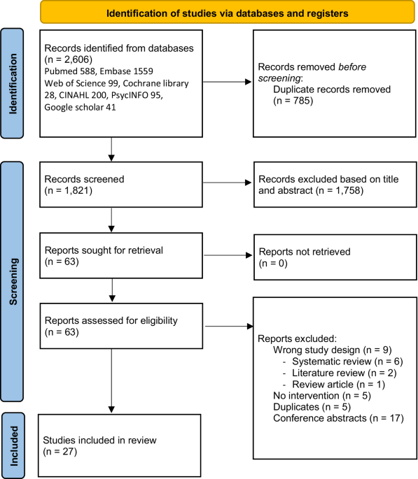
Sample multiplexing allows multiple samples to be pooled and sequenced simultaneously, resulting in lower per-sample sequencing costs19. However, multiplexing may also increase the number of false positive variant calls20. To assess sequencing quality, we first compared the DP and variant calling when using WES without and with multiplexing of 4 and 8 samples (no-plexing, 4-plexing and 8-plexing, correspondingly). For this, we generated 37 exome sequences at 100X WES and different levels of multiplexing using DNA from Ashkenazi trio samples (Fig. 1, Supplementary Figure 1 and Methods).

Fig. 1: WEGS experimental design overview.

DNA samples from a GIAB family trio (HG002, HG003, HG004) were used to perform WES experiments without and with multiplexing of 4 and 8 samples (no-plexing, 4-plexing and 8-plexing, correspondingly). For each sample in the family trio, we performed library preparation and sequencing to a target coverage of 100X in triplicate for the no-plexing and 4-plexing WES experiments, and in duplicate for the 8-plexing experiment, for a total of 37 samples. Sequencing library QC was performed before and after exome capture. After libraries QC, three individual libraries – one from each sample in the family trio - were selected to perform low-depth WGS on two lanes. Sequencing was performed using the Illumina NovaSeq S1 platform.

We observed a strong negative correlation (Pearson’s r = −0.69, P value = 2.31 × 10−6) between the average DP in targeted exome regions and the number of multiplexed samples (Fig. 2). The median values of average DP across individual exomes dropped from 121.8 in no-plexing experiments to 98.6 and 82.6 in 4-plexing and 8-plexing, respectively. The average DP ratio between no-plexing and 4- and 8-plexing experiments was similar in all targeted regions across the exome - showing no evidence that differences in average DP were non-uniform or affected only a subset of targeted regions (Supplementary Fig. 2). When stratifying by library preparation batch, we observed statistically significant differences (P value = 0.048) in average DP between two batches only in experiments without multiplexing (Supplementary Fig. 3A). Nevertheless, these differences did not influence the overall trend - the strong negative correlations between the number of multiplexed samples and DP remained in both library preparation batches (Supplementary Figure 3B–C).

Fig. 2: Average depths of coverage across all targeted regions in autosomal chromosomes in WES experiments without and with multiplexing.

The average depth of coverage (DP) was computed across target regions in Agilent V7 capture using paired mapped reads and counting only base-pairs with minimal Phred-scaled mapping and base qualities of 20. The solid black line corresponds to the linear regression line, and the dashed black lines correspond to a 95% confidence interval. The box bounds the IQR, and Tukey-style whiskers extend to a maximum of 1.5 × IQR beyond the box. The horizontal line within the box indicates the median value. Open circles are data points corresponding to the average DP across individual exome.

To better understand the cause of lower average DP in multiplex sequencing, we assessed the total number of paired reads, the number of reads flagged as PCR or optical duplicates, the number of unmapped reads, and the average base qualities in reads. There was no correlation (Pearson’s r = −0.08, P value = 0.631) between the total number of paired reads and the number of samples pooled together for sequencing (Supplementary Figure 4A). However, there was a strong positive correlation (Pearson’s r = 0.92, P value = 2.13 × 10−15) between the percent of reads flagged as PCR or optical duplicates and degrees of multiplexing (Supplementary Figure 4B). Compared to the multiplexing-free sequencing experiments, the 4-plexing and 8-plexing experiments showed a 1.7-fold (18.4% vs 31.2%) and 2.3-fold (18.4% vs 43.0%) increase in the median percent of duplicated reads, respectively. The data also suggested a weak, non-statistically significant correlation (Pearson’s r = 0.32, P value = 0.06) between the percent of unmapped reads and degrees of multiplexing (Supplementary Figure 4C). Also, the percent of unmapped reads did not exceed 0.11 percent of the total number of paired reads and, thus, did not contribute much to the differences in average DP. There was a moderate correlation (Pearson’s r = −0.52, P-value = 1.09 × 10−3) between the average base qualities and the degree of multiplexing (Supplementary Fig. 4C). However, when stratified by the library preparation batch and in contrast to the other metrics mentioned above, the first batch did not show the same correlation pattern (Supplementary Figs. 5–8), suggesting that other factors may affect the base qualities. We conclude that the main contributor to the lower average DP in sample multiplexing experiments compared to the experiments without sample multiplexing is the percent of reads flagged as PCR or optical duplicates.

UMI does not recover losses in the depth of coverage

UMI - a unique barcode appended to each DNA fragment before the PCR - helps to distinguish the truly duplicated fragments originating from the same molecule from the very similar fragments originating from a different molecule21,22. In addition, UMI-aware software tools for duplicate read removal help to identify and remove sequencing errors by grouping reads with the same UMI and creating a consensus read23. We applied the duplex UMI method in our sequencing experiments and evaluated the utility of LocatIt and UmiAwareMarkDuplicatesWithMateCigar (GATK + UMI) UMI-aware read deduplication tools with multiplexing. LocatIt reduced the average DP in experiments without and with multiplexing, compared to the UMI agnostic deduplication approach, while UMI + GATK increased the average DP (Supplementary Figure 9). We explain the different effects on average DP by the difference in strategies between these two tools. For example, in 8-plexing experiments, the GATK + UMI reduced the percent of duplicated reads on average by 0.4 (SE = 0.01), while LocatIt reduced it by 1.56 (SE = 0.03) (Supplementary Table 2). However, LocatIt, on average, marked an additional 4.38% of reads as QC failed, which included reads with low base qualities in their UMIs and single consensus read pairs without complementary pairs. This additional filtering in LocatIt resulted in lower average DP, fewer unmapped reads, and higher average base qualities. In summary, the UMI-aware read deduplication showed that the vast majority of the duplicated reads in multiplexing experiments are truly PCR/optical duplicates. UMI-aware deduplication didn’t help recover the loss in average DP in multiplexing experiments back to the levels of no-plexing experiments.

Sample multiplexing decreases variant recall rates

We observed moderate-to-strong negative correlations between the number of samples sequenced together and the recall rates for SNVs (Pearson’s r = −0.60, P value = 7.79 × 10−5) and InDels (Pearson’s r = −0.48, P value = 2.85 × 10−3) (Supplementary Figure 10A, C). The average recall rates dropped from 0.983 (SE = 0.0004) and 0.939 (SE = 0.003) in no-plexing experiments to 0.980 (SE = 0.0004) and 0.926 (SE = 0.003) in 8-plexing experiments for SNVs and InDels, respectively (Supplementary Table 3). In many instances, the recall rates were lower in the second library preparation batch, and some of these differences were statistically significant (Supplementary Figure 11A, D). Despite these differences, the statistically significant negative correlations between variant recall rates and the number of multiplexed samples were present in both library preparation batches (Supplementary Figure 11B, C, E, F).

We also observed a drop in precision for both variant types with the increased number of multiplexed samples, but unlike recall, the negative correlations were weaker and not statistically significant (Supplementary Figure 10B, D, Supplementary Table 3). The precision rates were similar between the library preparation batches (Supplementary Figure 12A, D), and they also did not show statistically significant correlations with the number of multiplexed samples when stratified by batch (Supplementary Figure 12B, C, E, F). Only in the first batch we saw a weak positive correlation (Pearson’s r = 0.27, P value = 0.26) between precision and the number of multiplexed samples (Supplementary Figure 12B).

We looked into the number of true positive (TP), false positive (FP), and false negative (FN) variant calls to explain the statistically significant decrease in recall rates. We found the strongest correlation in the degree of multiplexing and the number of FN calls (Pearson’s r = 0.60, P value = 8.46 × 10−5 in SNVs and Pearson’s r = 0.44, P value = 6.34 × 10−3 in InDels), representing the true variants that are not detected (Supplementary Figure 13). For example, the average number of undetected true SNVs increased from 384 (SE = 8) in single-sample sequencing experiments to 446 (SE = 9) in 8-plexing experiments (Supplementary Table 3). On average, 65 (SE = 6) true SNVs missed in 8-plexing experiments were correctly identified across all no-plexing experiments for the corresponding sample, and 61 (SE = 6) of those had a higher depth of coverage in no-plexing experiments than in 8-plexing experiments (Supplementary Table 4). We conclude that the main driver for the decrease in recall rates is the drop in average DP in multiplexing experiments, which leads to the increased number of missed true variants.

UMI improves variant calling insufficiently

We investigated how the recall and precision rates changed in SNV calling after applying the UMI-aware duplicate read removal. We wanted to test if a more accurate read deduplication could partially compensate for the loss of variant recall rates in multiplexing experiments. As previously, we considered two UMI-aware deduplication tools: LocatIt and UmiAwareMarkDuplicatesWithMateCigar (GATK + UMI).

We observed small but statistically significant drops in the recall rates when using LocatIt in all samples at all levels of plexing (Supplementary Figure 14A). For example, on average, the paired difference in the same sample in the 8-plexing experiment between two recall rates, one measured after LocatIt and another measured after the UMI agnostic approach, was only −0.0008 (SE = 0.0001) (Supplementary Table 5). The paired differences between the recall rates were consistently negative in all samples in the 8-plexing experiment, and this relationship was statistically significant (P value = 2 × 10−3) (Supplementary Figure 14A). However, there was no consistent and statistically significant change in the precision rates: precision slightly increased in some samples but dropped in others (Supplementary Figure 14B). For instance, while, on average, a paired difference in the 8-plexing experiment between precision rates increased by 0.0002 (SE = 0.0002) (Supplementary Table 5), the paired differences between precision rates were negative in 5 out of 16 samples and did not support this average increase (P value = 0.85) (Supplementary Figure 14B). The statistically significant decreases and increases were also in the total number of called SNVs and the number of missed true SNVs (i.e. FN calls), respectively (Supplementary Table 5). In samples in the 8-plexing experiments, the average paired difference between the total numbers of called SNVs was −20 (SE = 4) and between the numbers of missed true SNVs was 17 (SE = 2). Although the average paired difference between the numbers of FP calls was −2 (SE = 3) and suggested a decrease in the numbers of FP calls when using LocatIt, this relationship was not statistically significant (P-value ≥ 0.05). The reduced number of called SNVs is consistent with our previous observation of reduced average DP when using LocatIt due to additional read filtering.

When using GATK + UMI, we observed slight but statistically significant improvements in the SNV recall rates for samples in multiplexing experiments (Supplementary Figure 14C). In samples in the 8-plexing experiments, the average paired difference between recall rates was 0.0003 (SE < 0.0001) (Supplementary Table 5), and the increase in recall rates was observed in the majority of samples and supported the statistical significance of the relationship (P value = 3.1 × 10−5) (Supplementary Figure 14C). At the same time, there was also a slight statistically significant drop in the precision rates at all levels of plexing (Supplementary Figure 14D). In the same samples in the 8-plexing experiments, the average paired difference between precision rates was −0.0014 (SE = 0.0001) (Supplementary Table 5), and the decrease was consistent across all samples leading to the statistically significant relationship (P-value = 1.5 × 10−5) (Supplementary Table 5). The observed increase in the number of called SNVs (e.g. M = 39 [SE = 2] in 8-plexing) and the number of FP calls (e.g. M = 33 [SE = 2] in 8-plexing) with a much smaller decrease in the number of FN calls (e.g. M = −6 [SE = 1] in 8-plexing) (Supplementary Table 5) can explain the increase in recall and decrease in precision rates. The increase in the number of called SNVs is consistent with our previous observation of increased DP when using GATK + UMI.

In summary, while UMI-aware read deduplication can improve SNV recall or precision rates depending on the approach, this improvement appears minimal in the present experiment. It does not allow to recover these rates back to levels similar to no-plexing experiments.

WEGS significantly improves variant calling in multiplexed samples

To compensate for the losses in variant recall rates when performing multiplexed WES, we introduced reads from low-depth WGS before variant calling. We called this approach WEGS. We evaluated four combinations in comparison to no-plexing WES: (1) 4-plexing WES and WGS at 2X average DP (WEGS4P,2X), (2) 4-plexing WES and WGS at 5X average DP (WEGS4P,5X), (3) 8-plexing WES and WGS at 2X average DP (WEGS8P,2X), and (4) 8-plexing WES and WGS at 5X average DP (WEGS8P,5X). In each combination, we looked at the paired difference in the same sample between two recall rates, one measured after adding reads from WGS and another before.

Additional reads from 2X and 5X WGS improved variant recall rates in all multiplexing experiments, and the differences were statistically significant (P value < 0.05) (Supplementary Figures 15 and 16). For instance, the average paired difference in SNV recall rates in WEGS8P,2X was 0.0031 (SE = 0.0002) (Supplementary Table 6). This paired difference in recall rates was positive across all samples and, thus, supported the statistical significance of the observed increase in recall rates (P value = 1.5 × 10−5) (Supplementary Figure 15A). The total number of discovered SNVs increased on average by 76 (SE = 6), of which 70 (SE = 5) were true positives, explaining the improved recall rates (Supplementary Table 6). Similarly, there were statistically significant improvements in InDel recall rates (Supplementary Figures 15C and 18C). As expected, adding reads from 5X WGS improved the recall rates the most. The average paired difference in SNV recall rates in WEGS8P,5X was 0.0044 (SE = 0.0003) compared to 0.0031 (SE = 0.0002) in WEGS8P,2X (Supplementary Table 6).

The change in variant precision rates after adding reads from low-depth WGS differed for SNVs and InDels. We observed slight drops in SNV precision rates in all combinations of multiplexing levels in WES and read depths in WGS. However, the declines were not systematic, i.e. they were present only in part of the samples, in contrast to increases in SNV recall rates which were, on average, much higher and present in all samples (Supplementary Figures 15B and 16B). For example, the lowest average paired difference in SNV precision rates among all WES and WGS combinations was −0.0003 (SE = 0.0001) in WEGS4P,2X (Supplementary Table 6). It was the only combination where this paired difference in SNV precision rates reached statistical significance (P value = 0.026) (Supplementary Figure 15B). Thus, adding reads from low-depth WGS increased the number of called SNVs by a few dozen, but at the same time, some of these additionally called SNVs were FP, which slightly changed the SNV precision rate in either direction.

Differently from SNVs, all combinations of multiplexing levels in WES and read depths in WGS showed statistically significant improvements in InDel precision rates (P value < 0.05). In WEGS8P,2X, the average paired difference in InDel precision rates was 0.0055 (SE = 0.0009) (Supplementary Table 6), and only 1 out of 16 pairs had a negative paired difference between InDel precision rates after and before adding WGS reads (Supplementary Figure 15). In contrast to SNVs, additional reads from 2X WGS raised the average number of called InDels by 10 (SE = 2) and, at the same time, decreased the average number of FPs by 6 (SE = 1) in 8-plexing WES.

WEGS enhances WES with millions of variants genome-wide

We compared the variant recall rates in standard no-plexing WES to those in multiplexing WES combined with low-depth WGS (Fig. 3A, C). The average SNV and InDel recall rates exceeded the corresponding rates in no-plexing WES for most WEGS configurations, except for WEGS8P,2X. Both WEGS4P,2X and WEGS4P,5X resulted in higher average SNV recall rates than no-plexing WES: 0.9842 (SE = 0.0002, P value = 6.4 × 10−3) and 0.9852 (SE = 0.0001, P value = 7.1 × 10−5) against 0.9830 (SE = 0.0004), respectively (Fig. 3A). Among 8-plexing experiments, only WEGS8P,5X resulted in higher average SNV recall rates than no-plexing WES: 0.9847 (SE = 0.0001, P-value = 5.6 × 10−4). Similarly, only WEGS4P,2X, WEGS4P,5X, and WEGS8P,5X statistically significantly increased average InDel recall rates compared to no-plex WES (Fig. 3C). The average InDel recall rate showed a statistically significant increase from 0.9390 (SE = 0.0029) in no-plex WES to 0.9493 (SE = 0.0029, P value = 0.01), 0.9552 (SE = 0.0019, P value = 2.8 × 10−4), and 0.9490 (SE = 0.0020, P value = 4.2 × 10−3) in WEGS4P,2X, WEGS4P,5X, and WEGS8P,5X, respectively. When stratified by the library preparation batch, the average variant recall rates across WEGS remained higher than those in no-plexing WES, except for SNV recall rates in WEGS8P,2X (Supplementary Figures 17E, F, 18E, F). The batch effect in SNV recall rates in WES, described above, also affected WEGS (Supplementary Figure 18D). Despite this, the WEGS4P,5X and WEGS8P,5X had statistically significantly higher SNV recall rates compared to no-plexing WES in both batches, and the increase in WEGS4P,2X was close to statistical significance (Supplementary Figure 17E, F). There were no statistically significant differences in InDel recall rates between the two batches within the no-plexing WES and each WEGS configuration (Supplementary Figure 18D). But only for WEGS4P,5X the increase in InDel recall rates compared to no-plexing WES was statistically significant in both batches. WEGS4P,2X showed a statistically significant increase only in the first batch. WEGS8P,2X showed a statistically significant increase only in the second batch, and the increase in the first batch was close to a statistical significance (P-value = 0.092).

Fig. 3: Variant recall and precision rates in no-plexing WES and WEGS.

The figure represents variant calls inside the target regions in Agilent V7 capture and the GIAB high-confidence regions. The box bounds the IQR, and Tukey-style whiskers extend to 1.5 × IQR beyond the box. The horizontal line within the box indicates the median value. Open circles are data points corresponding to the individual WES and WEGS. The p-values above each sequencing method pair correspond to the one-tailed Wilcoxon rank-sum test. A Recall rates of the called SNVs. B Precision rates of the called SNVs. C Recall rates of the called InDels D Precision rates of the called InDels. Supplementary Table 6 shows average values and standard errors.

The variant calling precision rates in no-plexing WES compared to WEGS differed depending on the variant type. The average SNV precision rates in every WEGS configuration were slightly lower than in WES, while average InDel precision rates were higher than in WES (Fig. 3B, D, Supplementary Table 7). Only drops in average SNV precision rates in WEGS4P,2X and WEGS4P,5X, and an increase in the average InDel precision rate in WEGS4P,5X were statistically significant (Supplementary Table 7). Furthermore, when stratified by the library preparation batch, the decreases in average SNV precision rates in WEGS compared to no-plexing WES were statistically significant only in the second batch (Supplementary Figure 17A–C, Supplementary Table 8). In contrast, WEGS8P,2X and WEGS8P,5X demonstrated an increase in average SNV precision rates compared to no-plexing WES in the first batch. We explain this by the initially lower precision rates in multiplexing WES experiments in the second batch as described above. When stratified the average InDel recall rates by the library preparation batches, the average InDel precision rates in WEGS remained higher than in no-plexing WES for all configurations except WEGS8P,2X (Supplementary Figure 18A–C, Supplementary Table 8). However, none of the increases remained statistically significant.

We also compared variant recall and precision rates in WES and WEGS to the 30X WGS, which we generated by downsampling reads from 300X WGS data (see Methods). Average variant recall and precision rates inside regions targeted by WES were higher in 30X WGS compared to WES and WEGS. For SNVs, these differences were below 0.7%, while for InDels, the maximal difference reached 6% (Supplementary Table 9). WEGS4P,2X, WEGS4P,5X, and WEGS8P,5X were closer to 30X WGS than WES in targeted regions. 30X WGS had no rivals when comparing genome-wide recall and precision rates. On average, it found 1.7–2.5 times more SNVs and 2.5–3.8 times more InDels genome-wide than WEGS (Supplementary Table 10). The average genome-wide SNV and InDel precision rates in WGS were up to 18% and 70% higher than in WEGS, respectively. As expected, WEGS4P,5X and WEGS8P,5X were the closest to the 30X WEGS.

In summary, these results confirm that our WEGS approach eliminates the negative impact of sample multiplexing in WES on variant recall rates in coding regions and brings variant recall rates to the levels of a standard no-plexing WES or higher. Furthermore, these results suggest that WEGS4P,2X, WEGS4P,5X and WEGS8P,5X are the closest alternatives to no-plexing WES, as these sequencing strategies demonstrated statistically significant increases in SNV and InDel recall rates and, at the same time, showed increases in InDel precision rates in targeted regions. WEGS has a clear advantage over WES by allowing the assessment of additional ~2 M SNVs and InDels per individual genome-wide.

WEGS correctly assesses variants which genotype imputation misses

Next, we wanted to understand what other benefits low-depth WGS data could bring to multiplexed WES besides removing the negative effects of sample multiplexing. We compared WEGS to array-based genotyping followed by genotype imputation. For each of our three samples, HG002, HG003, and HG004, we emulated the genotyping array data covering 654,013 genetic positions and performed genotype imputation using the TOPMed reference panel consisting of 97,256 diverse genomes. We compared these imputation results to WEGS4P,2X and WEGS8P,5X, the closest alternatives to no-plexing WES in targeted regions.

First, we investigated regions targeted by WEGS. SNVs imputed from emulated genotyping array data showed high precision rates ( > 99%) for all three samples, but imputation missed between 824 to 1,028 SNVs per sample (among them, between 482 to 576 were non-synonymous) compared to WEGS (Supplementary Table 11). For example, in sample HG002, WEGS8P,5X correctly identified 22,390 SNVs on average, and the TOPMed reference panel imputed only 21,458 SNVs, which is 938 SNVs less. The difference in the number of correctly identified InDels was even larger: imputation missed around 60% of true InDels (40% recall), while WEGS only missed around 5% (95% recall).

Second, we investigated the number of imputed and sequenced variants genome-wide (Supplementary Table 12). In contrast to the WEGS targeted regions, the genotyping array-based imputation approach outperformed WEGS by the number of correctly identified SNVs: imputation missed 4–5% (95–96% recall), WEGS4P,2X missed 54–65% (35–46% recall), and WEGS8P,5X missed 36–50% (50–64% recall) of true SNVs. The differences in correctly identified InDels were much lower: imputation missed around 61% (39% recall), WEGS4P,2X missed 69–78% (22–31% recall), and WEGS8P,5X missed 53–67% (33–47% recall) of true InDels.

Third, we looked at how many variants missed or wrongly imputed outside non-protein coding regions can be recovered by WEGS. We grouped TOPMed-imputed variants outside WEGS-targeted non-protein-coding regions into three categories: (1) the number of imputed alleles matches the number of true alleles (i.e. imputation is correct); (2) the number of imputed alleles is less than the number of true alleles; (3) the number of imputed alleles is higher than the number of true alleles. For each of these groups, we looked at the median fold change in alternate AF between the ASJ population and TOPMed. The median fold-change in AF was higher (i.e. AF in ASJ was higher than in TOPMed) when imputation was systematically missing alleles (group 2) and lower when imputation was wrongly imputing extra allele(s) (group 3) (Supplementary Table 13). This result is in line with previous studies24,25, which showed that the imputation accuracy depends on the genetic similarity between the study individual and the reference panel. WEGS4P,2X correctly identified true alleles in 38–46% of variants in group 2 and 89–92% of variants in group 3, while WEGS8P,5X correctly identified true alleles in 55–67% of variants in group 2 and 91–94% in group 3.

Finally, to improve the variant recall in non-coding regions in WEGS, we evaluated the applicability of the GLIMPSE method26, developed to impute missing variants from low-depth WGS data. After applying GLIMPSE to WEGS4P,2X and WEGS8P,5X with local reference haplotypes from the 1000 Genomes Project and Human Genome Diversity Project (see Methods), genome-wide SNV recall rates and precision increased drastically. In imputed WEGS4P,2X, the average genome-wide SNV recall rate and precision increased from ~35–46% to ~69–81% and from ~80–82% to ~94–95%, respectively (Supplementary Tables 12 and 14). In imputed WEGS8P,5X, the average genome-wide SNV recall rate and precision increased from ~50–65% to ~79–89% and from ~87–90% to ~95–96%, respectively. The genome-wide recall rate and precision also increased for InDels. When considering the GLIMPSE-imputed variants only, i.e. without merging them with variants called in sequencing data only, the SNVs precision rate was very high and greater than 99% across all sequencing experiments (Supplementary Table 15). The SNV recall rate in sequence-based imputation was still lower than in genotyping array-based imputation. One of the possible explanations is that the state-of-the-art TOPMed reference panel contains >20 times more haplotypes than our local reference panel. To confirm this, we run the genotyping array-based imputation using our local reference panel and the Minimac4 tool27. The Minimac4-imputed recall rates for SNVs were only slightly higher than the GLIMPSE-imputed WEGS8P,5X and much higher than the GLIMPSE-imputed WEGS8P,2X (Supplementary Table 16). However, the precision rates of GLIMPSE-imputed SNVs were always much higher than those of the Minimac4-imputed SNVs. When considering imputed variants only, the recall rates for imputed InDels were similar in the sequence-based imputation and genotyping array-based imputation using TOPMed, but were lower compared to genotyping array-based imputation using the local reference panel. The InDels recall rates became closer to Minimac4-imputation results when combining imputed and called InDels together, but at the expense of precision.

In summary, these results showed that WEGS outperforms the genotyping array and imputation approach in terms of the number of identified variants, especially InDels, inside protein-coding regions. Outside protein-coding regions, WEGS allows one to discover genetic variants missed by genotyping array-based imputation due to their population specificity. Sequencing-based imputation methods can be applied to WEGS to recover variants missed due to lower depth of coverage outside protein-coding regions. WEGS8P,5X has a clear advantage over WEGS4P,2X outside the protein-coding region due to the higher depth of coverage in the WGS experiment.

WEGS is substantially cheaper than high-depth WES and WGS

We compared costs for WEGS scenarios relative to genotyping arrays, low-depth WGS, 30X WGS and no-plexing 100X WES. Per sample cost estimates for the genotyping array included DNA QC and genotyping using Affymetrix Axiom UKBB array. Sequencing costs per sample were based on current pricing and a scenario of 1,000 samples sequenced on the Illumina NovaSeq 6000, S4 platform. We note that sequencing costs can vary depending on multiple factors, including reagents pricing, flow cell volume and sequencing platform, while genotyping array prices are less affected by sample size.

Our estimates show that the combinations of WEGS4P,2X and WEGS8P,5X are half the price compared to standard 100X WES (no-plexing) and ~47% of the price of 30X WGS (Table 1). The combination of 5X WGS with 4-plexing WES is slightly more expensive but still 56% of the cost of 30X WGS and 60% of the cost of no-plexing 100X WES. As such, the WEGS scenarios representing the most economical strategies relative to WGS and WES are again the combinations of 2X WGS with 4-plexing WES and 5X WGS with 8-plexing WES. Yet, as shown above, while WEGS4P,2X and WEGS8P,5X show comparable precision and recall in targeted coding regions relative to standard WES, the latter combination is more effective at capturing noncoding variation. As such, we conclude that the most cost-effective WEGS strategy to capture both coding and non-coding variants is 5X WGS with 8-plexing high-depth WES.

Table 1 Relative genotyping and sequencing costs per sample given current pricing.WEGS applied to the study of peripheral artery disease

We applied WEGS8P,4X to 862 patients diagnosed with PAD. Based on the genetic ancestry analyses (see Methods), 780 (90.5%) PAD patients were inferred as Europeans, 60 (7.9%) as Admixed Americans, 7 (0.8%) as Africans, 4 (0.6%) as Asians and 3 (0.3%) as middle Eastern (Supplementary Figure 19). The GIAB control sample included in each of the 10 plates showed similar precision and recall for SNVs and InDels as in the benchmark experiment (Supplementary Figure 20). After variant level filtering (see Methods), we identified 44,747,114 genetic variants (33,505,105 SNVs and 11,242,009 InDels) in PAD samples (Table 2). A total of 12,893,703 of these variants were novel (not described in dbSNP v109.3), from which 63.8% were singletons (carried by one individual). Inside the coding regions, we observed 35.4% synonymous (11,053 per individual), 59.0% non-synonymous (11,636 per individual), 1.1% stop/essential splice (490 per individual), 2.1% frameshift (298 per individual), and 2.3% (371 per individual) inframe genetic variants.

Table 2 The number of variants discovered in WEGS sequencing data from 862 patients with peripheral artery disease.

We evaluated the WEGS ability to capture known loci associated with PAD identified by large-scale GWAS28. All lead variants mapping to these loci were present in the PAD WEGS data (Supplementary Table 17). The majority of the lead variants are intergenic, with an average read depth of 13.7. Only 6 out of the 19 lead variants are directly typed onto the Global Screening Array (GSA) 24.v3; demonstrating the WEGS potentials to assess disease-causing variants beyond the genotyping arrays. In addition, we observed that WEGS captured, on average, 4056 (SE = 295) genetic variants within the known PAD loci that are not present in the TOPMed imputation reference panel and, thus, could not be imputed (Supplementary Table 18). Although the majority of these loci are intergenic, WEGS was able to identify additional missense variants within these regions.