Scanner geometry

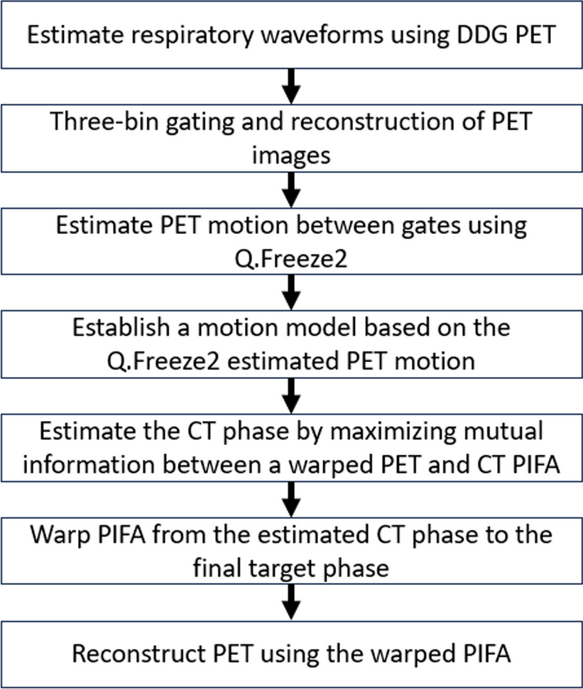
The DMI is a silicon photomultiplier-based PET/CT scanner, with lutetium-yttrium oxyorthosilicate (LYSO) crystals. Partial description of the geometry of different DMI PET systems have already been reported [26,27,28,29]. In this work, the geometry of the DMI 4-ring (including crystal/module spacing) and the detectors configuration (indexing) have been modelled according to the data provided by the manufacturer. In GATE, the rsector is the largest geometry inside the cylindricalPET, and a total of 34 rsectors were arranged to form the scanner ring. Each rsector contained four modules, adjacent in the axial direction. In each module, four blocks were stacked, containing a \(4 \times 9\) array of LYSO crystals. The crystals dimensions were 5.3 (axial) \(\times ~3.95\) (transaxial) \(\times ~25\) (length) mm\(^3\). Overall, this geometry gave a 20-cm axial FOV and a 70-cm transaxial FOV. The rsectors’ lead shielding and the inner plastic cover were also modelled. Figure 1 shows the visual representation of the DMI model in GATE, without the patient bed. When the patient bed was used in experimental acquisitions, it was also included in the associated GATE simulations.

Fig. 1

a GATE representation of the DMI 4-ring with the rsectors (34 in totals) in blue, the lead shielding in cyan and the detector covers in grey and b the structure of a rsector

Simulation environment/framework

GATE 9.0 and Geant4 10.5 were used to model the DMI. The GATE physics list was set to \(emstandard\_ opt\) and no custom cuts or variance reduction techniques were used, i.e. all particles were generated and tracked according to the default behaviour defined in Geant4. The radioactive source was set to \(\beta +\) emissions for all simulations, where setForcedUnstableFlag was used to ensure source decay with setForcedHalfLife 6586.2 s. The \(^F\) branching ratio to \(\beta +\) was reproduced by multiplying the desired 18F source activity by 0.969 in the GATE simulation. The energy of the \(\beta +\) source was set according to the Landolt-Börnstein tables available in GATE (energytype Fluor18). The simulations were performed on the Centre de Calcul de l’Université de Bourgogne (CCUB) using computers with Intel Xeon Gold CPU 6126 @ 2.60 GHz and 64 GB memory. To speed up GATE simulations, each simulation was equally divided into n sub-simulations with \(t_ = t_/n\); where \(n\in \mathbb \), tsubsimulation is the simulation time of each sub-simulation and tsimulation is the simulation time of the whole GATE simulation. Our simulations were performed with \(200\le n \le 400\), depending on the expected simulation time.

All NEMA tests were analysed using in-house tools implemented in Python/C++. They were validated by comparing the experimental results processed using these tools with those obtained using the manufacturer’s software tools (see Appendix “Simulation environment/framework”). However, as the time-of-flight resolution test was not available in the manufacturer’s software for our Generation 1 (Gen1) DMI 4-ring, the results of our in-house tool were compared with published data obtained from a Generation 2 (Gen2) DMI 6-ring (see “Time-of-flight resolution”).

Data processing

When performing acquisitions on the DMI, experimental data could either be stored in list mode or in three-dimensional (3D) sinograms. The list mode data could then be rearranged in 3D sinograms using a proprietary offline reconstruction package, hereafter referred to as the PET toolbox (GE HealthCare, Chicago, Il, USA). The output of a GATE simulation provides a list mode with single and coincidence events, stored as a Python NumPy array. This list mode includes the exact position of the annihilations, and the type of each coincidence (i.e. true, random, or scatter). Simulated list modes were organised into 3D sinograms using GATE detector numbers and look-up tables provided by the manufacturer. The 3D sinograms were of dimensions 415 (radial bins) × 1261 (planes) × 272  (projections). The TOF sinograms were of dimensions 1261 (planes) × 29 (time) × 415 (radial bins) × 272 (projections).

Image reconstruction

Image reconstruction of clinical data was done using the PET toolbox. It includes reconstruction algorithms such as filtered back-projection (FBP) and ordered-subsets expectation-maximisation (OSEM). Standard correction methods (implemented by the manufacturer) are provided within the PET toolbox: normalisation, decay, well-counter (calibration for quantification), attenuation, deadtime, random and scatter corrections [30,31,32,33].

In order to reconstruct simulated data, a specific interface has been added to the PET toolbox, allowing corrections for normalisation, attenuation, randoms and scatters. Currently, it does not support corrections for decay, deadtime and well-counter. This interface requires not only the sinograms to be reconstructed, but also calibration files for normalisation correction (geometrical factors and individual detector efficiencies), and an attenuation map for attenuation correction. The normalisation correction was performed according to a component-based method [34, 35]. To determine geometrical factors (each detector has the same detection efficiency in the model), two simulations were run at very high statistics where only true coincidences were recorded. The first simulation was performed with an annulus source of 32 cm radius, of 1 mm thickness, and 20 cm long, centred on the FOV of the scanner, where 3.2 billion true coincidences were collected over 253 CPU days of simulation. The normalisation factors were calculated with the help of a second simulation, using a flood source of 10 cm radius and 22 cm height positioned at the centre of the FOV, where 562 million of true counts were collected. This simulation took 137 CPU days to complete. The simulated attenuation map was generated in GATE using the MuMap actor. The output image contained the spatial distribution of the linear attenuation coefficient at 511 keV for the given study. Its dimensions and resolution were 256 × 256 × 71 pixels and 2 × 2 × 3 mm3, respectively. For the DMI, the estimation of random coincidences is performed on single events [30]. The proposed randoms from singles (RFS) formula shown in Eq. 1 has been applied to estimate random counts of the simulated data. For two given detectors x and y and their associated singles count rates \(s_x\) and \(s_y\), the estimated randoms rate between the two detectors \(r_\) is:

$$\begin r_=(2\tau )s_xs_y \end$$

(1)

where \(2\tau\) is the coincidence window size. Finally, scatter correction was performed using a model-based algorithm as implemented in the PET toolbox for clinical data  [32]. Overall, the proposed methodology allows a close comparison between experimental and simulated data, as the sinograms have the same properties and the reconstruction algorithms and corrections used were similar to the clinical setup.

NEMA studies

In this work, the NEMA NU 2-2018 [19] tests performed experimentally on the DMI scanner were compared with those simulated in GATE with the corresponding DMI model.

Sensitivity

A 700 mm-long, 1 mm inner diameter line source inserted into a 1.25-mm thick aluminium sleeve was filled with 3.3 MBq of 18F-FDG at the beginning of the acquisition and centred in the FOV. Five 60-second frames were acquired, successively increasing the number of aluminium sleeves around the source. Five more frames were acquired with the line source located at a radial offset of 10 cm from the centre. Simulations were strictly mimicking the experimental conditions. In both cases, 3D sinograms were rebinned into 2D sinograms using single-slice rebinning (SSRB) [36] and processed according to NEMA specifications. The system sensitivity (counts/sec/MBq) and the axial sensitivity profile were reported.

Scatter fraction, count losses, and randoms

Noise equivalent counts (NEC) and scatter fraction (SF) were computed according to NEMA using a 18F-FDG line source inserted into a cylindrical polyethylene phantom of 700 mm length and 101.5 mm radius. The line source had an inner diameter of 3.2 mm and a length of 700 mm. The activity at the start of the acquisition was 719 MBq. This phantom was built geometrically in GATE following the NEMA specifications, and the patient bed was also modelled.

Experimentally, 24 frames were acquired during ten hours: 17 contiguous acquisitions of 15 min, followed by seven acquisitions of 25 min, spaced 25 min apart. These long acquisitions, coupled with very high activity, could not be fully simulated in GATE, because the CPU time and computing power required would have been excessive. Therefore, the duration of the simulated acquisitions were set to obtain at least ten million prompts per frame, while maintaining the same number of frames and average activities.

Experimental and simulated data were rebinned into two-dimensional (2D) sinograms using SSRB and processed according to NEMA specifications.

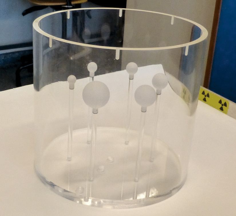
Spatial resolution

The NEMA spatial resolution test was acquired on the DMI using two sets of three 18F-FDG point sources placed at 1, 10, and 20 cm from the FOV centre in the radial direction. One set was located in the central transverse plane of the scanner and the other at an offset of three-eighths of the axial FOV (i.e. 76 mm) from the FOV centre. In GATE, spheres of 0.5 mm radius were used to simulate the six point sources. The duration of the experimental and simulated acquisition was 60 s.

In both cases, the image reconstruction was performed using the same implementation of the FBP algorithm with a ramp filter and a cut-off at the Nyquist frequency (no smoothing). The reconstruction was centred on the sources with a transverse FOV of 250 mm so as to reach a voxel size of 0.65 × 0.65 × 2.79 mm3.

Time-of-flight resolution

For this test, the experimental and simulated data acquired during the count losses test (see “Scatter fraction, count losses, and randoms”) were used.

On DMI 4-ring Gen1 systems, the detection of coincidences is performed with a time resolution sampling S of 13.02 ps, but the obtained TOF list mode data are further mashed by a factor C of 13, resulting in a final sampling resolution of \(CS = 169.26\) ps. Although this compression does not penalise the reconstruction of TOF data (the Nyquist–Shannon sampling theorem is respected), it has a major impact when using the NEMA method to evaluate the TOF resolution.

To process these mashed data, each 169.26 ps bin was uniformly resampled over 13 bins of 13.02 ps, and the TOF resolution of the system CTRmash was estimated according to the NEMA guidelines. To account for the degradation of the CTR due to mashing, an empirical correction factor was then applied to obtain the final result CTRcor, assuming Gaussian-distributed data:

$$\begin }_ = \sqrt}_^ - \left[ 2\sqrt}(2)} \times \frac}\right] ^2} \end$$

(2)

In this expression, the term in square brackets represents the uncertainty contribution induced by the use of mashed data in the NEMA process:

\(2\sqrt\) is the term used to obtain a Gaussian full width at half maximum (FWHM) from its standard deviation,

\(CS/\sqrt\) is the derived global standard deviation of the uncertainty introduced by the mashing and the processing steps. It is the quadratic sum of the errors associated with (i) the mashing of a uniformly sampled distribution [0, CS] by a factor C, (\(CS / \sqrt\)), and (ii) the uniform up-sampling from CS-sized bins to S-sized bins (\(CS / \sqrt\)).

The same process was applied to the simulated data: the raw TOF data from GATE were mashed over 169.26 ps bins, then processed according to the NEMA guidelines to obtain the simulated CTRmash and the simulated CTRcor according to Eq. 2.

To determine the line source position, the experimental data were reconstructed using OSEM with all available corrections except decay correction. A 3D line was fitted to the centroid of each reconstructed axial plane, and the associated unit vector was computed using the intersection of this fit with the first and last axial planes. The simulated line source unit vector was determined based on the position of the phantom in GATE.

The timing error analysis was performed to obtain a TOF offset profile for experimental and simulated data by processing 20 million and 10 million counts, respectively. The TOF offset profile was corrected for scatters and randoms according to the NEMA report.

Image quality, accuracy of corrections

The image quality test was performed on the DMI with an IEC NEMA body phantom which contained 5.3 kBq/mL and 20.9 kBq/mL of 18F-FDG in the background and spheres, respectively, resulting in a 3.9:1 sphere-to-background ratio (SBR). The body phantom was centred in the FOV so that the middle of the spheres was at the centre of the axial FOV. According to NEMA, the NEC phantom (see “Scatter fraction, count losses, and randoms”) was placed on the patient bed outside the imaging FOV, aligned with the body phantom, and the line source was filled with approximately 120 MBq of 18F-FDG. Three repeated acquisitions were launched with decay-adjusted times of acquisition. Image quality analysis was performed according to NEMA for these three acquisitions and then averaged to obtain the final experimental results.

In GATE, an IEC NEMA body model was built geometrically following the NEMA specifications. The patient bed and the 700 mm-long cylindrical phantoms were also modelled. All phantom positions were set to replicate the experimental setup. Simulated data were collected over a single simulation of 270 s.

Acquired experimental and simulation data were reconstructed using the OSEM algorithm, with TOF information (TOFOSEM). Two iterations and 17 subsets were used with a 6.4-mm Gaussian filter in the transverse direction and a 3-point filter in the Z-axis (defined as standard). Scatter, random, attenuation, and normalisation corrections were performed. All reconstructed images had a size of 256 × 256 × 71 pixels, with a pixel size of 2.73 × 2.73 × 2.79 mm, covering a FOV of 700 mm. To assess the impact of corrections on the simulated data, an additional reconstruction, where the prompts were perfectly-corrected of random and scatter counts (i.e. only true counts were reconstructed), was performed and analysed.

The reconstructed images were evaluated in terms of contrast recovery coefficient (CRC), background variability (BV) and residual lung error (LE) as per NEMA guidelines. The image roughness (IR) [37] was also investigated.

Electronics modelling/signal processing

In GATE, the digitiser handles the signal processing of the photons, from photonic hits in crystals to coincidences. It consists of several modules that can be tuned through their associated parameters in order to accurately model the electronic chain of a PET system. Figure 2 shows the signal processing chain formed by the different modules of the DMI’s GATE model. Photonic hits are added into pulses, which are then processed into singles, to finally obtain coincidences.

The following sections describe the digitiser modules and the methods used to determine their optimal parameter values. The raw data acquired in “Scatter fraction, count losses, and randoms” were used to evaluate the system’s single, prompt and random rates over a wide activity range, between 0.8 and 31.2 kBq mL−1. For this purpose, experimental and simulated counts were obtained from list mode and sinograms, without additional data processing, to ensure proper initial modelling of the DMI in GATE.

Fig. 2

The complete digitiser model of the DMI 4-ring. In blue are the different modules with their associated parameters values. The orange dashed box encapsulates the processing of hits, the purple one the processing of pulses, and the last red box the processing of singles into coincidences

Readout

After hits in a given volume are summed together into pulses by the adder module, pulses are then grouped by the readout module. The policy takeEnergyCentroid has been used with setDepth 1, positioning the summed pulses by weighting the crystal indices of each pulse by the deposited energy (Anger-logic scheme).

Energy and temporal windows/resolutions

The energy window, energy resolution, and coincidence timing window (CTW) parameter values have been set according to the manufacturer’s specifications [38]. The coincidence time resolution (CTR) parameter value has been set according to experiments performed on our DMI 4-ring, using the methodology proposed by Uribe et al. [39]. Using this method, a value of 375 ps was measured, which is in line with the values reported in the literature by other groups for the DMI 4-ring [26, 29, 40]. Energy thresholding is the final step in the signal processing of singles events and its lower and upper bounds were set at 425 keV and 650 keV, respectively. The energy resolution was set to 9.4% at 511 keV for all crystals. While the time resolution is usually defined in terms of CTR, GATE accepts only singles timing resolution (STR). As CTR is assumed to follow a Gaussian distribution, the associated FWHM can be used to find the STR as follows: STR = CTR/\(\sqrt\), giving STR = 0.265 ns. The coincidence window size in GATE represents the size of the window opened by an incoming single event. Since the nominal CTW value of the DMI system is \(2\tau =4.9\) ns, the value \(\tau =2.45\) ns was set in the digitiser.

Background noise and quantum efficiency

The background noise and quantum efficiency can be determined by following the method proposed by Salvadori et al. [41], using the experimental single counts Sexp acquired during the NEMA count losses test. These experimental counts were compared to simulated singles counts Ssim acquired under the same conditions, with simulation deadtime, background noise (Noisesim), and quantum efficiency (QEsim) ignored, i.e. removed from the digitiser. The low-activity data of both acquisitions (supposed to be unaffected by deadtime) were then used to fit a linear model according to (3), so as to determine QEsim and Noisesim. Using this method, a background noise of 1193 kHz and a quantum efficiency of 97.75% were found for the DMI.

$$\begin S_= }_ (S_ + }_) \end$$

(3)

Singles deadtime and pile-up

At high activity, count rates are impacted by two main non-linear effects: deadtime and pile-up. Photon detection losses induced by pile-up are linked to energy thresholding. On one hand, the stacking of two single events can move the signal of a photon within a true coincidence outside the energy window (diminishing the rate of true coincidences). On the other hand, it can also move the signal of a scattered photon inside the energy window (increasing the rate of scattered coincidences). Therefore, the pile-up value impacts the true-to-scatter ratio, and it must be modelled before energy discrimination. Deadtime can be modelled either before or after the energy window, with no subsequent impact on the true-to-scatter ratio. When modelled after the energy window, it enables the use of an experimentally determined value. If modelled before the energy window, an optimisation process is required.

Therefore, the balance between the deadtime and pile-up values is guided by the trues count rate provided by the GATE model. It can be determined using the NEMA count losses methodology applied to the simulated data used in section “Background noise and quantum efficiency”. For our model, the simulated true count rate was higher than the experimental true count rate, even at low activities. In this work, the pile-up value was determined through empirical optimisation, using the prompt count rates obtained during the NEMA count losses analysis. Simulations were performed by varying the pile-up values so as to obtain the best fit between experimental and simulated prompt rates, and a value of 20 ns was found to be optimal.

Coincidence sorting

After energy thresholding, the resulting singles are grouped into coincidences in a CTW of 4.9 ns (see “Energy and temporal windows/resolutions”). By setting the allPulseOpenCoincGate parameter to true, we ensured that each single opens its own coincidence window, whether or not a window is already opened. Multiple coincidences were handled using the takeAllGoods policy as this has been suggested to give the best coincidence matching to MC data for most PET system designs [42]. In addition, all coincidences had to satisfy a geometric condition to restrict coincidence formation within a given transaxial FOV. This is handled by the minSectorDifference parameter, which was set to four, resulting in a 70 cm transaxial FOV.