Here, we detail the dataset used in the creation of the docking pipeline as well as the dataset employed for evaluation of our pipeline. We describe the creation of inter-pose similarity statistics by performing cross-docking on a diverse protein-ligand benchmark dataset. The Open-ComBind docking pipeline is described, harnessing the similarity statistics to performing pose selection on a ligand of interest, the ‘docking ligand’, using a set of ligands with unknown bound structures, the ‘helper ligands’. Finally, an experiment to determine the validity of Open-ComBind’s underlying hypothesis: ‘distinct ligands bind to a receptor in similar ways’.

DataSimilarity dataset

Following [18], a list of 30 target proteins (Table S1) representative of all major families of drug targets is used to generate the pairwise pose feature similarity distributions. The entire benchmark dataset of 421 protein-ligand pairs is used to generate the similarity statistics.

Benchmark dataset

Generating the dataset used for evaluating pose prediction pipelines necessitates removal of easy-to-dock ligands. Following [18], we filter the Similarity Dataset to remove any ligand that has greater than 50% of its atoms in the maximum common substructure computed with the cognate ligand of the receptor structure used for docking. If a new ligand shares most of the same structure as the cognate ligand then its probable the pocket has an appropriate configuration to bind the similar ligand. This reduces the set to 245 protein-ligand complexes for determining the performance of a pose prediction pipeline. These ligands are used as the ‘docking ligand’ during the evaluation of the pipeline.

Helper ligands

Helper ligands are a set of ligands known to bind to the receptor of interest with \(<1\mu M\) affinity, but may not have a solved bound structure. These ligands are used along with the ‘docking ligand’ in the Open-ComBind pipeline to improve pose selection of both the ‘docking ligand’ and the ‘helper ligands.’

We utilize the same two sets of helper ligands as in [18]: one in which the helper ligands do not share a scaffold with the docking ligand, termed ‘High-affinity helper ligands’, and the other in which the ligands have the largest Maximum Common Substructure (MCSS) with the docking ligand, termed ‘Congeneric series helper ligands’. We use the MCSS definition from [18] to ensure we are using the same set of helper ligands.

Derivation of similarity distributions

Here we detail the development of pairwise similarity distributions for near-native poses and all docked poses using the Similarity Dataset.

Protein and ligand pre-processing

Protein and ligand pre-processing separates the protein and ligand into separate docking-ready structures. Initially, a set of co-crystallized protein-ligand structures for each receptor in the Similarity Dataset is downloaded from RCSB.org [21, 22]. The ligand of interest in each co-crystallized structure is then designated based on its residue name. Using ProDy [19, 20], separate files are generated for the protein, ligand, waters, and other heteroatoms that are present in the original crystal structure. The instance coordinates of the ligand structure are downloaded directly from RCSB.org [21, 22] using their File Download Service to ensure proper coordinate and bond information. Using only the protein and ligand complex, we align all structures of a receptor based on the residues closest to the binding pocket. Protein residues within 15 Å of the ligand are used to align each receptor structure with PyMol [23] to the alphabetically lowest PDB ID (PDB IDs specified in Table S1). The co-crystallized ligand’s coordinates are transformed according to the receptor alignment object. The aligned ligand and receptor are then separated into their own files to provide a ground-truth ligand and a holo structure for cross-docking with non-cognate ligands. After removal of the ligand, missing residues, atoms, and hydrogens are added (at a pH of 7.0) to the receptor structures using PDBFixer and minimized, ensuring interactions are detected properly after docking. Missing atoms and hydrogens are minimized using the default OpenMM forcefield. Finally, a gnina docking command template is created for each protein. The gnina docking command template specifies the docking protein structure (i.e. the aligned-to receptor structure) as well as the binding box location, defined by the cognate ligand of the docking receptor.

Docking with gnina requires knowledge of the 3D structure of the ligands to be docked. Conformations are generated for ligands using Experimental-Torsion with basic Knowledge Distance Geometry (ETKDG) [24, 25] to yield likely conformations of the ligand based on trends seen in crystal conformations. Using RDKit, we generate 50 conformations, and use the Universal Force Field (UFF) to minimize and report the energy of each generated conformation. Combining the ten lowest energy conformations into a single file for each ligand. A set of low-energy conformations gives a higher likelihood that one of the conformations is close to the ground-truth ligand conformation. Additionally, gnina docking keeps rigid bond angles and lengths, so using multiple conformations of a ligand during docking allows for exploration of different bond angles and lengths.

Cross-docking

After both ligand and protein preparation, cross-docking is performed with gnina. All of the ligands are docked against the receptor structure used for the alignment, the alphabetically lowest PDB ID (Table S1). The receptor’s cognate ligand identifies the binding site. Docking is performed using all default parameters, except for exhaustiveness, min_rmsd_filter, and num_modes (Table S2). exhaustiveness is increased to 16 to perform more sampling of the ligand during docking. min_rmsd_filter is reduced to 0.01 to allow highly similar, high-scoring poses to be output. num_modes is set to 30 to ensure we have a max number of 300 total poses for each ligand if we have ten starting conformations for each ligand. Following the docked pose statistics of [18], which have up to 300 poses per docked ligand, we attempt to sample 300 docked poses per ligand complex. Additionally, gnina tends to produce distinct poses in comparison to Glide which tends to output highly similar poses, often leading to generating several near-native poses. Therefore, we utilize several ligand conformations during docking to increase the likelihood that gnina outputs more than one pose close to the native state. After docking, we re-sort the combined output poses from gnina for each ligand according to the ‘CNNscore’, a score in the range [0,1] denoting the likelihood a ligand pose is correct [26]. Following [18] and to reduce computation, only the top 100 docked poses of each ligand are used for subsequent steps.

Featurization

The top 100 docked poses of each ligand are investigated for their interactions with the receptor and their distance from the ground truth, if available. Each pose has associated docking scores from both Autodock Vina and the Convolutional Neural Network (CNN) scoring functions in gnina. Additionally, the interaction fingerprint of each docked pose is computed. The interaction fingerprint profiles and scores the hydrogen bonds, salt bridges, and hydrophobic contacts between the protein and ligand. Hydrogen bond scores are a product of the distance between the donor and the acceptor’s hydrogen and the angle between the donor, hydrogen, and acceptor. However, since gnina ignores hydrogens in both the input and output, we add hydrogens to the docked poses with RDKit and minimize the hydrogen atom placement with UFF, ignoring the effect of the protein environment. Both the salt bridge and hydrophobic contact scores are simply the distance between the involved atoms. Unique to Open-ComBind, salt bridges are determined via ligand substructure matches to SMARTS strings, taken from Pharmit [27], for the detection of positive and negative ions rather than using atoms with a formal charge since gnina does not modify the formal charge of the input molecule based on the receptor environment. These scores are summed by protein residue for each feature type.

Following the featurization of individual poses, we can calculate the similarity of pairs of poses based on their features. A pseudo-Tanimoto Similarity is used for the similarity of hydrogen bonds, salt bridges, and hydrophobic contacts. Since the features are not bit vectors, the Tanimoto Similarity between pose i and j is calculated as follows:

$$\begin \mathrm TS_ = \frac}} \sqrt \sqrt}}} \sqrt \sqrt} \end$$

where f is one of the features and \(}\) are all of the residues of the docking protein. An additional inter-pose feature is calculated via the RMSD between the MCSS of the two poses. We utilize a set of MCSS parameters that find a substructure with both matching atom IDs and bond orders. However, halogen atoms are allowed to match any other halogen atoms and rings are constrained to only match other, complete rings. We do not consider the MCSS if the number of heavy atoms in the MCSS is less than half the number of heavy atoms in the smallest ligand.

Generating similarity statistics

Given our inter-pose features, we can now compute the extent to which ligands binding to the same receptor do so in a similar manner. We first define the ‘native distribution’, which looks at the inter-pose similarity between only poses with < 2Å RMSD from the ground truth, denoted as \(f(s(\cdot ,\cdot )|\,\text )\). We next define the ‘reference distribution’ to be the inter-pose similarity between all pairs of the top 100 poses output by gnina, denoted as \(f(s(\cdot ,\cdot )|\,\text )\). Both distributions are determined via a Gaussian kernel density estimate on each of the inter-pose features. Following [18], the Gaussian kernel density estimate uses a standard deviation of 0.03 for interaction similarities and 0.18 for MCSS RMSD. Reflected boundaries are used to reduce bias near the boundaries.

The distributions for MCSS RMSD were both capped at 6 Å to eliminate the effect of the sparse distribution for higher RMSDs. Any values greater than 6 Å were set to 6 Å.

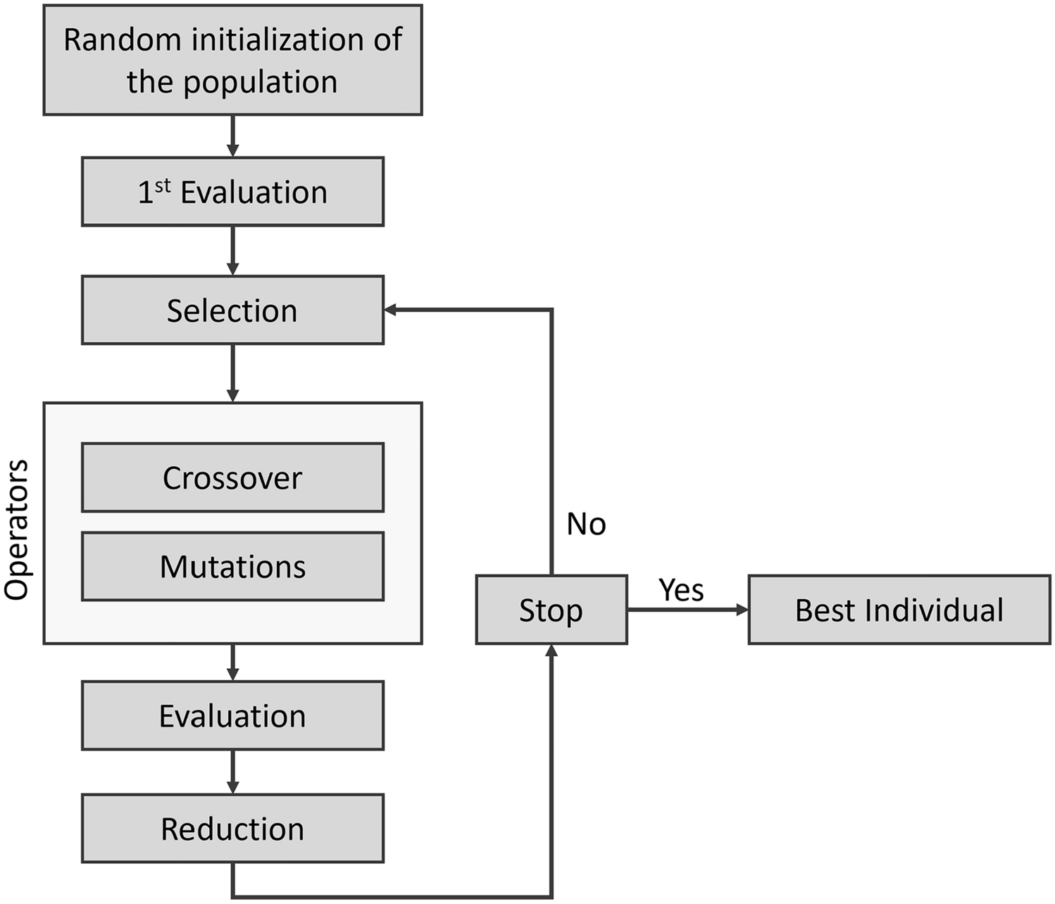
Open-ComBind pose prediction pipelineFig. 1

Open-ComBind pose prediction pipeline: the user provides a docking ligand, a holo receptor structure, and a defined binding pocket on the structure. The user can then define a set of helper ligands: molecules with \(<1\mu M\) affinity to the receptor but not requiring any bound structure. A set of conformations is generated for the docking ligand and the helper ligands. gnina is used to dock the docking and helper ligands, outputs are sorted by CNNscore. The poses for each ligand are featurized and inter-pose similarities are calculated between all pairs of poses. Finally, the poses for the docking ligand as well as the helper ligands are selected using the Open-ComBind objective function which harnesses the pre-computed similiarity distributions

Open-ComBind provides a pipeline (Fig. 1) that prepares protein and ligand structures for docking, a suite of methods to compute the similarity of features from pairs of docked ligands, as well as predicting a set of poses utilizing pre-computed similarity distributions. Protein-ligand ground-truth complexes, usually determined via X-ray crystallography, are manipulated to extract separate protein and ligand structures after alignment of the pocket residues of similar protein structures. Ligands are prepared for docking by generating a set of low-energy 3D ligand conformations. Docking is run on a single receptor conformation with all of the generated conformers per ligand and the output for each ligand is sorted according to its docking score. Featurization of the top poses for each ligand includes their docking score and fingerprint of the protein-ligand interactions. Feature similarities are computed between all pairs of ligand poses, both inter- and intra-ligand pairs, utilizing the pose interaction fingerprints and the RMSD between the MCSS of the pose pair. We use the same protein and ligand pre-processing, conformation generation, docking, and featurization procedure as enumerated in “Derivation of similarity distributions” section. Finally, a pose is selected for each docked ligand by maximizing the sum of the similarity between the pose selected for each ligand and the pose’s docking score.

Poses are selected for the docking ligand and the set of helper ligands utilizing the inter-pose features in tandem with the pre-computed native and reference distributions. Adhering to the same procedure as [18], we randomly initialize pose selections and randomly iterate through the ligands, picking a pose that maximizes the objective:

$$\begin & }_} = -C\cdot \text (\ell _i) \\ & \quad + \frac\sum \limits _}}\sum \limits _\log \frac)})} \end$$

where \(\ell _i\) is the pose selected for the current ligand, \(}\) is our set of similarities, \(f(s(\cdot ,\cdot )|\,\text )\) and \(f(s(\cdot ,\cdot )|\,\text )\) refer to the pre-computed native and reference similarity distributions, respectively, and C is a hyperparameter to weight the CNNscore. We attempt to identify the set of selected poses that optimizes this objective function through a greedy iterative process. We continue iterating through the ligands, updating the selected pose, until no new poses are selected for any ligands. This procedure is run 500 times to increase the likelihood of finding the global minimum. The poses selected by the objective function for each ligand are returned.

Selection of CNNscore weight

We select the hyperparameter, C, for the weight of the CNNscore (the pose score output by gnina [26]) within the Open-ComBind score function in the same way as [18]. The same cross-docked top 100 poses for each ligand used for computing the similarity statistics are pooled and sorted according to their CNNscore. For each consecutive cluster of 100 poses, we calculate the average CNNscore and the negative log-likelihood of those 100 poses being a correct pose (i.e. \(\le 2\)Å from the ground truth). A line is fit to the data and the slope is used as the weight for the CNNscore.

Benchmark dataset evaluation

Cross-docking is the main focus of many docking studies as it most closely emulates docking experiments in drug discovery campaigns. We test the performance of Open-ComBind by performing cross-docking on the Benchmark Dataset. We utilize the protein and ligand pre-processing available in the Open-ComBind pipeline to prepare the ligands for cross-docking. A protein and ligand file are created for each complex of the Benchmark Dataset, however, binding site cofactors are manually added back to the protein, following ComBind’s preparation procedure for a fair comparison. Next, we create two sets of helper ligands for each ligand we are docking, as defined above: high-affinity binders and congeneric series. We then use the Open-ComBind Pose Prediction Pipeline (Fig. 1) on each ligand in which we are performing cross-docking with each set of helper ligands. When predicting poses for docking ligands of a given receptor, we omit that receptor’s docked ligand similarity statistics from the pre-computed similarity statistics used in the Open-ComBind objective function.

We run the evaluation, for each docking ligand, using five different random seeds to determine the variability of Open-ComBind given slightly different ligand poses. The random seed are used for the creation of the conformations of the docking ligand and helper ligands as well as the gnina docking procedure.

Hypothesis evaluation

[18] built ComBind on the hypothesis that distinct ligands bind to a receptor in similar ways. We aim to investigate whether this underlying hypothesis of the pipeline is correct by comparing the value of the Open-ComBind objective function for the lowest RMSD ligand poses to the value of the objective when selecting from all gnina generated poses. We only look at target proteins in the Benchmark dataset containing at least ten ligands with a gnina generated near-native pose. In the following experiment, we only use ligands with a defined ground truth pose (i.e. the set of docking ligands for each target receptor in the benchmark dataset) and only ligands that have a gnina generated pose < 2Å RMSD from the ground truth. We first measure the value of the Open-ComBind objective function when we restrict our selection to the best gnina generated pose, according to lowest RMSD to the ground truth. We next evaluate the value of the Open-ComBind objective function when we select from all gnina generated poses of the ligands. If the underlying hypothesis of Open-ComBind is true, then the Open-ComBind objective function value when selecting from the best poses will be greater than or equal to the objective function value when selecting from all gnina generated poses. The Open-ComBind objective is optimized in a stochastic manner, so it is possible we will not converge on the globally optimal pose selections which is assumed to be the set of poses with the lowest RMSD to the ground truth.