1 Introduction

Drivers driving for a long time or driving at night can lead to a decline in physical and psychological abilities, seriously affecting the ability to drive safely. Fatigue while driving can impair basic skills such as attention, decision-making, and reaction time, while also affecting cognitive processes, sensory perception, and overall mental well-being. In severe cases, this may result in a decline in motor function and increase the likelihood of being involved in traffic accidents. Statistically, in 2004, the World Health Organization released the “World Report on Road Traffic Injury Prevention”, which pointed out that approximately 20%~30% of traffic accidents were caused by fatigue driving. By 2030, the number of road traffic fatalities is projected to rise to about 2.4 million people annually, making road traffic deaths the fifth leading cause of death worldwide (WHO, 2009). As the number of casualties due to fatigue driving continues to increase, it is urgent to develop reliable and effective driving fatigue detection methods.

The existing fatigue detection methods mainly include vehicle information-based, facial feature-based, and physiological signal-based approaches. The vehicle information-based detection method indirectly assess the driver's fatigue state based on the driver's manipulation of the vehicle (Li et al., 2017; Chen et al., 2020). This method utilizes on-board sensors and cameras to collect data such as steering wheel angle, grip force, vehicle speed, and driving trajectory. By analyzing the differences in driving behavior parameters between normal driving and fatigue states, it assesses the driver's fatigue condition. However, it is challenging to collect accurate and stable data using this method due to variations in driving habits and proficiency among drivers. The facial feature-based detection method infers the driver's fatigue state through analyzing eye status, mouth status, and head posture (Wu and, 2019; Quddus et al., 2021; Huang et al., 2022). This method mainly uses the camera to capture the driver's face image, and extracts the fatigue-related information through the computer vision technology. In contrast, physiological signal-based detection methods can directly reflect the driver's driving state, including electroencephalogram (EEG), electrooculogram (EOG), electrocardiogram (ECG), and electromyogram (EMG). Among various physiological signals, EEG signals contain all the information of brain operation and are closely related to mental and physical activity, with good time resolution and strong anti-interference ability (Yao and Lu, 2020), which are the result of excitatory or inhibitory postsynaptic potentials generated by the cell bodies and dendrites of pyramidal neurons (Zeng et al., 2021). Meanwhile, the EEG caps tend to be intelligent and lightweight (Lin et al., 2019), making it convenient to keep an EEG cap while driving. EEG signals are considered the most direct and promising.

EEG signals are recordings of the spontaneous or stimulus-induced electrical activity generated by specific regions of the brain's neurons during physiological processes, reflecting the brain's biological activities and carrying a wealth of information (Jia et al., 2023). From an electrophysiological perspective, every subtle brain activity induces corresponding neural cell discharges, which can be recorded by specialized instruments to analyze and decode brain function. EEG decoding is the separation of task-relevant components from the EEG signals. The main method of decoding is to describe task-related components using feature vectors, and then use classification algorithms to classify the relevant features of different tasks. The accuracy of decoding depends on how well the feature algorithm represents the relevant tasks and the discriminative precision of the classification algorithm for different tasks. The EEG signals record the electrical wave changes in brain activity, making them the most direct and effective reflection of fatigue state. Based on the amplitude and frequency of the waveforms, EEG waves are classified into five types: δ(1-3Hz), θ(4-7Hz), α(8–13Hz), β(14–30Hz), γ(31–50Hz) waves (Song et al., 2020). It is worth noting that, during the awake state, EEG signals are mainly characterized by α and β waves. As fatigue increases, the amplitude of α and β waves gradually diminishes, and they may even disappear, while δ and θ waves gradually increase, indicating significant variations in EEG signals during different stages of fatigue (Jia et al., 2023). Therefore, many scholars regard EEG signals as the gold standard for measuring the level of fatigue (Zhang et al., 2022). Lal and Craig (2001) tested non-drivers' EEG waves and analyzed the characteristics of EEG wave changes in five stages: non-fatigue, near-fatigue, moderate fatigue, drowsiness, and anti-fatigue. They concluded that EEG is the most suitable signal for evaluating fatigue. Lal and Craig (2002) collected EEG data from 35 participants in the early stage of fatigue using 19 electrodes. The experimental results indicated a decrease in the activity of α and β waves during the fatigue process, while there was a significant increase in the activity of δ and θ waves. Papadelis et al. (2006) introduced the concept of entropy in a driving fatigue experiment. The study found that under severe fatigue conditions, the number of α waves and β waves exhibited inconsistent changes, and shannon entropy and kullback-leibler entropy values decreased with the changes in β waves.

In recent years, thanks to the rapid development of sensor technology, information processing, computer science, and artificial intelligence, a large number of studies have proposed combining fatigue driving detection based on EEG signals with machine learning or deep learning methods. Paulo et al. (2021) proposed using recursive graphs and gramian angular fields to transform the raw EEG signals into image-like data, which is then input into a single-layer convolutional neural network (CNN) to achieve fatigue detection. Abidi et al. (2022) processed the raw EEG signals using a tunable Q-factor wavelet transform and extracted signal features using kernel principal component analysis (KPCA). They then used k-nearest neighbors (KNN) and support vector machine (SVM) for EEG signal classification. Song et al. (2022) proposed a method that combines convolutional neural network (CNN) and long short-term memory (LSTM) called LSDD-EEGNet. It utilizes CNN to extract fe atures and LSTM for classification. Gao et al. (2019) introduced core blocks and dense layers into CNN to extract and fuse spatial features, achieving detection. In the study (Wu et al., 2021), designed a finite impulse response (FIR) filter with chebyshev approximation to obtain four EEG frequency bands (i.e., δ, θ, α, β), and constructed a new deep sparse contracting autoencoder network to learn more local fatigue features. Cai et al. (2020) introduced a new method referred to as graph-time fusion dual-input convolutional neural network. This method transforms each EEG epoch of sleep stages into limited penetration visible graph (LPVG) and utilizes a new dual-input CNN to assess the degree sequences of LPVG and the original EEG epochs. Finally, based on the CNN analysis, the sleep stages are classified into six states. Gao et al. (2021) were the first to explore the application of complex networks and deep learning in EEG signal analysis. They introduced a fatigue driving detection network framework that combines complex networks and deep learning. The network first calculates the EEG signals for each channel and generates a feature matrix using a recursive rate. Then, this feature matrix is fed into a specially designed CNN, and the prediction results are obtained through the softmax function.

The above deep learning and convolutional neural network (CNN) methods mainly focus on the features of individual electrode EEG signals and overlook the functional connectivity of the brain, that is the correlation between EEG channels. Due to the non-Euclidean structure of EEG signals, CNN based on Euclidean space learning is limited in handling the functional connections between different electrodes. Therefore, using CNN to process EEG signals may not be an optimal choice.

In recent years, the emergence of graph convolutional neural networks (GCN) has been proven to be the most effective method for handling non-Euclidean structured data (Jia et al., 2021; Zhu et al., 2022). Using GCN to process EEG signals allows to represent the functional connections of the brain through topological data. In this case, each EEG signal channel is treated as a node in the graph, and the connections between EEG signal channels serve as the edges of the graph. Jia et al. (2023) proposed a model called MATCN-GT for fatigue driving detection, which consists of a multi-scale attention time convolutional neural network block (MATCN) and a graph convolution-transformer (GT) block. The MATCN directly extracts features from the raw EEG signals, while the GT processes the features of EEG signals from different electrodes. Zhang et al. (2020) introduced the PDC-GCNN method for detecting driver's EEG signals, which uses partial directed coherence (PDC) to construct an adjacency matrix, and then employs graph convolutional neural network (GCN) for EEG signal classification. Song et al. (2020) proposed a multi-channel EEG emotion recognition method based on dynamic graph convolutional neural network (DGCNN). The basic idea is to use graphs to model multi-channel EEG features and then perform EEG emotion classification based on this model. Jia et al. (2020) proposed a novel deep graph neural network called GraphSleepNet to classify EEG signals. This network can dynamically learn the adjacency matrix and utilizes a spatio-temporal graph convolutional network (ST-GCN) to classify EEG signals. The method demonstrated excellent classification results on the MASS dataset. Zhang et al. (2019) designed a graph convolution broad network (GCB-net) to explore deeper-level information in graph-structured data. It utilizes graph convolutional layers to extract features from the input graph structure and stacks multiple regular convolutional layers to capture more abstract features. Additionally, a broad learning system (BLS) is employed to enhance the features and improve the performance of GCB-net.

Although GCN is proficient at learning the internal structural information of EEG signals, it relies on the connectivity between nodes provided by the adjacency matrix. Most methods obtain functional connectivity of EEG signals by using predefined fixed graphs such as PLI, PLV, PDC, or spatial relationships, which prevents the model from adaptively constructing adjacency graphs simultaneously related with subjects, fatigue states and samples, thereby overlooking the data-driven intrinsic correlations. However, constructing a suitable graph representation for the adjacency matrix of each data in advance requires time and effort. Additionally, GCN faces challenges in learning dependencies between distant nodes (long-range vertices). Increasing the depth of GCN to expand the receptive field remains difficult and may lead to over-smoothing of nodes.

To address the above problem, we propose a new fatigue driving detection network, referred to as the attention-based multi-semantic dynamical graph convolutional network (AMD-GCN). First, the network utilizes a channel attention mechanism based on average pooling and max pooling to assign weights to the fused EEG input features. This helps the model focus on the crucial information parts related to fatigue detection. Next, the adjusted EEG input features are fed into the GCN, we determine the adjacency matrix using spatial adjacency relationships, Euclidean spatial distances, and self-attention mechanism to construct data-driven intrinsic topology under multiple semantic patterns, thereby enhancing the spatial feature extraction capability of GCN. Furthermore, a spatial attention mechanism based on average pooling and max pooling is employed to calculate the weights of spatial nodes in the output of GCN, which helps in removing redundant node information and reducing interference in fatigue detection. Finally, the prediction results are output by softmax.

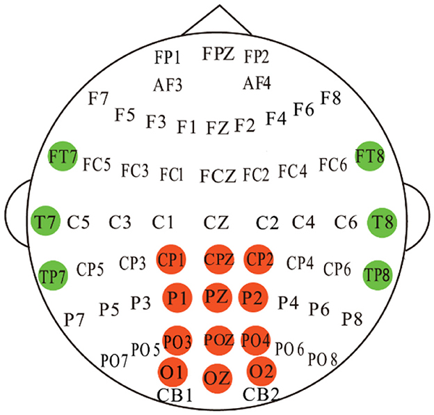
2 Dataset description and EEG pre-processing 2.1 Public dataset SEED-VIG

We validated the proposed method on the publicly available dataset SEED-VIG (Zheng and Lu, 2017) for driving fatigue detection researches. SEED-VIG adopt the international 10-20 electrode system standard, and the EEG signals were collected from 6 channels in the temporal region of the brain (FT7, FT8, T7, T8, TP7, TP8) and 12 channels from the posterior region (CP1, CPZ, CP2, P1, PZ, P2, PO3, POZ, PO4, O1, OZ, O2), where CPZ channel serves as the reference electrode, and the specific electrode placement is shown in Figure 1. The experiment simulated a driving environment by creating a virtual reality scenario, in which 23 participants engaged in approximately 2 hours of simulated driving during either a fatigue-prone midday or evening session. The subjects comprised 12 females and 11 males, with an average age of 23.3 years and a standard deviation of 1.4. All subjects had normal or corrected vision.

Figure 1. Electrode placements for the EEG setups. 12-channel and 6-channel EEG signals were recorded from the posterior region (red color) and the temporal region (green color), respectively.

The SEED-VIG dataset was vigilantly annotated using eye-tracking methods, capturing participants' eye movements with the assistance of SMI eye-tracking glasses. These glasses categorized eye states into fixation, blink, and saccade, and recorded their respective durations. The “CLOS” state, referring to slow or long-duration eye closure, is undetectable by the SMI eye-tracking glasses. In such cases, fixation and saccade represent normal states, while blink or CLOS indicates fatigue in participants. Therefore, PERCLOS represents the percentage of time in a specific period when participants were in a fatigued state (Dinges and Grace, 1998). The calculation of PERCLOS is as follows:

PERCLOS=blink+closeinterval,interval=blink+fixation+saccade+close    (1)

Where blink, close, fixation, and saccade denote the duration of eye states (blink, close, gaze, and sweep, respectively) recorded by the eye tracker within the 8-second intervals. PERCLOS is a continuous value between 0 and 1, with smaller values indicating higher vigilance. The standard procedure for using this publicly available dataset for research is to set two thresholds (0.35 and 0.7) in order to classify the samples into three types:

• Awake class: PERCLOS < 0.35;

• Tired class: 0.35 ≤ PERCLOS < 0.7;

• Drowsy class: PERCLOS ≥ 0.7.

In addition, we validated our proposed method on the SEED-VIG dataset, dividing each subject's 885 samples into 708 samples for training and 177 samples for testing by a way that preserves the temporal order, then we trained the model separately on each subject and evaluated it on the testing samples of the same subject. Finally, in order to mitigate the impact of data imbalance within one subject on the model performance evaluation as much as possible, the average classification accuracy and individual variation of 23 subjects were computed as evaluation metrics. It is worth noting that SEED-VIG adopts an 8-second non-overlapping sliding window to sample data, and we split the dataset by preserving the temporal order. Therefore, training is based on past data, and testing is based on future data. This ensures that the model is evaluated on unseen data, thereby alleviating the risk of data leakage (Saeb et al., 2017).

2.2 EEG pre-processing

The signal preprocessing method is consistent with other works (Zheng and Lu, 2017; Ko et al., 2021; Peng et al., 2023; Shi and Wang, 2023), we directly used the clean EEG signals provided by the study (Zheng and Lu, 2017), which has removed eye blinks, and the raw EEG data was downsampled from 1000 Hz to 200 Hz to reduce computational burden. Subsequently, it is bandpass filtered between 1-50 Hz to remove irrelevant components and power line interference. For SEED-VIG, there are two different methods to segment the frequency range into different bands. One widely used approach is to divide the frequency range into bands as follows: δ(1-3Hz), θ(4-7Hz), α(8-13Hz), β(14-30Hz), γ(31-50Hz). The other method is to uniformly divide the range into 25 bands with a 2-Hz resolution.

For each frequency band, the computation of the extracted differential entropy (DE) feature is as follows:

h(X)=-∫Xf(x)ln f(x)dx    (2)

Here, X is a random variable whose probability density function is defined by f(x). Assuming that the probability density function f(x) of the EEG signal follows the Gaussian distribution N(μ, δ2), the DE feature can then be computed as:

h(X)=-∫f(x)(-12ln (2πδ2)-(x-μ)22δ2)          =12ln (2πδ2)+Var(X)2δ2=12ln (2πeδ2)    (3)

Here, we used the facts that ∫ f(x)dx = 1 and Var(x) = ∫ f(x)(x − μ)2dx = δ2. DE features were extracted by short-term Fourier transform with an 8-second non-overlapping time window.

The overall properties of SEED-VIG are summarized in Table 1. In our study, we concatenate the DE features extracted based on 5 frequency bands and the DE features extracted based on 25 frequency bands within the same time window as one sample input to the neural network. This allows us to fully utilize the information contained in the original EEG signal and thereby enhance the effect of fatigue driving detection. The overall data form of one subject can be expressed as R885×17×30.

Table 1. Summary of the overall properties of SEED-VIG.

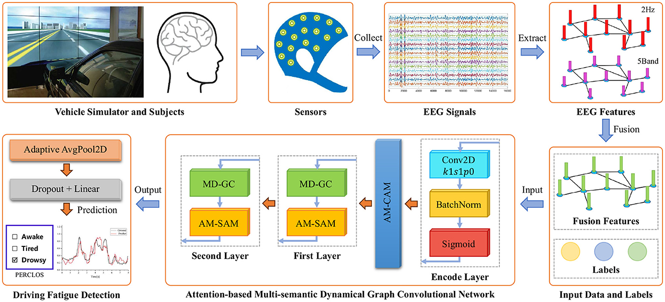
3 Method

Our proposed AMD-GCN model consists of three functional modules: channel attention mechanism based on average pooling and max pooling (AM-CAM), multi-semantic dynamical graph convolution (MD-GC), and spatial attention mechanism based on average pooling and Max pooling (AM-SAM). The AMD-GCN model enables end-to-end fatigue state assessment of drivers based on the extracted DE features from EEG signals. The AMD-GCN model retains crucial input features through AM-CAM, performs multi-semantic spatial feature learning through MD-GC, and eliminates redundant spatial nodes information through AM-SAM. The overall architecture of fatigue driving detection based on AMD-GCN is illustrated in Figure 2.

Figure 2. Overall schematic diagram of fatigue driving detection based on AMD-GCN. AMD-GCN consists of three modules: AM-CAM module, MD-GC module, and AM-SAM module. The input to the model is the fused feature of DE features extracted based on 5 frequency bands and DE features extracted based on 25 frequency bands. The output is the predicted label with probabilities.

3.1 Preliminary

In our paper, we designed the AMD-GCN model adopting graph convolutional neural networks to process spatial features. To facilitate reader comprehension, we first elucidate the fundamental concepts and relevant content of GCN before introducing AMD-GCN.

Consider a graph G = (V, ε, A), which represents a collection of all nodes and edges. Here, V = (v1, v2, ..., vn) signifies that the graph has N nodes, vn denotes the n-th node, and E is a set of edges representing relationships between nodes. A ∈ RN×N stands for the adjacency matrix of graph G, denoting connections between two nodes. It's worth noting that GCN (Kipf and Welling, 2016) employs graph spectral theory for convolutional operations on topological graphs. It primarily explores the properties of the graph through the eigenvalues and eigenvectors of the graph's Laplacian matrix. The Laplacian matrix of a graph is defined as follows:

where D ∈ RN×N is the degree matrix of the vertices (diagonal matrix), that is, the elements on the diagonal are the degrees of each vertex in turn. L denotes the Laplacian matrix, whose normalized form can be expressed as:

L=In-D-12AD-12=UAUT    (5)

Where In is the identity matrix. UAUT represents the orthogonal decomposition of the Laplacian matrix, where U=[u0,u1,...,un-1]∈Rn×n is the orthogonal matrix of eigenvectors obtained through the singular value decomposition (SVD) of the graph Laplacian matrix, and Λ=[λ0,λ1,...,λn-1]∈Rn×n is the diagonal matrix of corresponding eigenvalues. For a given input feature matrix X, its graph Fourier transform is:

X^=UTX,X=UX^(inverse)    (6)

The convolution of the graph for input X and filter K can be expressed as:

Y=X*GK=U((UTX)⊙(UTG))=UK^UTX    (7)

Here, ⊙ denotes the element-wise Hadamard product. However, directly computing the Eq.7 would require a substantial amount of computational resources. To mitigate energy consumption, Kipf and Welling (2016) proposed an efficient variant of convolutional neural networks that directly operate on graphs, approximating the graph convolution operation through a first-order Chebyshev polynomial. Supposing a graph G with N nodes, each node possessing its own features, let these node features form a matrix X ∈ RN×D. With an input feature matrix X and an adjacency matrix A, we can obtain the output:

Y=σ(D^-12AD^-12XW)    (8)

Where σ represents the nonlinear activation function.

3.2 Channel attention mechanism based on average pooling and max pooling

Firstly, we employ an autoencoder layer to perform re-representation of the input data, creating inputs with richer semantic information, as depicted in Figure 2, where the input channels are 30 and the output channels are 128. Then, in order to focus the model on crucial parts of the input related to the fatigue detection category, we generate channel attention maps by exploiting inter-channel relationships of features. This is achieved through the design of a channel attention mechanism based on average pooling and max pooling (AM-CAM) layer. The channel attention mechanism focuses on determining “what” in the input is meaningful, treating each channel of the feature map as a feature detector (Zeiler and Fergus, 2014). To compute channel attention effectively, we compress the spatial dimensions of the input feature maps. To gather spatial information, we employ an average pooling layer to gain insights into the extent of the target object effectively, utilizing it in the attention module to compute spatial statistics. Additionally, we use a max pooling layer to collect salient information about different object features, enabling the inference of finer channel attention. Figure 3 illustrates the computation process of channel attention maps, and the detailed operations are described as follows.

Figure 3. Schematic diagram of AM-CAM. As illustrated, the channel attention sub-module utilizes both the max pooling output and average pooling output with a shared network.

Given an intermediate feature map F ∈ RC×H×W as input, we first utilize average pooling and max pooling operations to aggregate spatial information from the feature map, generating two distinct spatial context descriptors: Favgc and Fmaxc, representing average-pooled features and max-pooled features, respectively. Subsequently, both of these descriptors are fed into a multilayer perceptron (MLP) with a hidden layer to generate the channel attention map Mc∈RC×1×1. To reduce parameter overhead, the hidden activation size is set to RCr×1×1, where r is the reduction ratio and is set to 16 in our study. After applying the shared network to each descriptor, we merge the output feature vectors using element-wise summation. In short, the channel attention is computed as:

Mc(F)=σ(MLP(AvgPool(F))+MLP(MaxPool(F)))             =σ(W1(W0(Favgc))+W1(W0(Fmaxc)))    (9)

Where σ denotes sigmoid function, W0∈RCr×C and W1∈RC×Cr, Note that the MLP weights, W0 and W1, are shared for both inputs and the ReLU activation function is followed by W0. The output Fout of AM-CAM can be formulated as:

Fout=Mc(F)⊙F    (10) 3.3 Multi-semantic dynamical graph convolution

In this study, we propose a multi-semantic dynamical graph convolution (MD-GC) for extracting spatial features from the input. It determines the adjacency matrix based on spatial adjacency relationships, Euclidean spatial distance, and self-attention mechanism. Our approach constructs data-driven intrinsic topology under various semantic patterns, enhancing the spatial feature extraction capability of graph convolution. Overall, given an intermediate feature map X ∈ RC×V as input, the output of MD-GC can be computed as:

MDGC(X) = σ(BN(SRGC(X) + EDGC(X)                    + SAGC(X)))    (11)

Where σ is sigmoid function, BN is batch normalization, SRGC represents spatial relationship-based graph convolution, EDGC represents Euclidean distance-based graph convolution, and SAGC stands for self-attention-based graph convolution.

3.3.1 Graph convolution based on spatial relationship

Intuitively, the correlation between EEG electrodes is constrained due to the distribution of nodes on the brain (Song et al., 2020), which represents inherent connections. To capture this relationship, we developed a spatial adjacency graph, denoted as GSR(V, ASR). ASR represents the spatial adjacency matrix between brain nodes, as shown in Figure 4, where adjacent nodes are connected by solid blue lines. ASR considers the adjacency relationships of 6 channels from the temporal region of the brain and 12 channels from the posterior part of the brain. We first normalize the spatial adjacency matrix ASR using

ÃSR=DSR-1ASR    (12)

DSR-1∈RN×N is a diagonal degree matrix of ASR. ÃSR provides nice initialization to learn the edge weights and avoids multiplication explosion (Brin and Page, 1998; Chen et al., 2018). Given the computed ÃSR, we propose the spatial relationship-based graph convolution (SRGC) operator. Let X ∈ RV×C and YSRGC∈RV×Cout be the input and output features of SRGC, respectively. The SRGC operator can be formalized as:

YSRGC=SRGC(X)=ÃSRXWSRT    (13)

Where WSR∈RCout×C is the trainable weight used to facilitate feature updating in the SRGC.

Figure 4. A schematic diagram illustrating the connections between the 17 EEG channels based on spatial adjacency relationships is used to construct the adjacency matrix for SRGC. CPZ serves as the reference electrode and is not involved in the construction of the adjacency matrix.

3.3.2 Graph convolution based on Euclidean-space distance

Considering that SRGC can only capture relationships between nodes connected by physiological connections, here we introduce a Euclidean distance-based graph convolution (EDGC) operator to capture potential relationships between physically non-connected nodes, thereby imposing higher-order positional information. Specifically, we define a Euclidean space distance adjacency matrix for the potential sample dependencies in EDGC, where the adjacency weight between nodes i and j is calculated as:

ai,j=max(E)-ei,j    (14)

where ei,j is an element at row i and column j in the matrix E ∈ RV×V that represents the distance between every pair of nodes. To calculate ei,j, we first assume the input takes the form of X ∈ RV×C. Then, we have ei,j=∥x̄i-x̄j∥2, where ∥x̄i-x̄j∥2 represents the Euclidean spatial distance between nodes i and j in X. Finally, subtracting ei,j from the maximum value in matrix E defines the adjacency relationship between nodes i and j, implying that nodes closer together have higher adjacency weights. Let YEDGC∈RV×Cout be the output features of EDGC, the EDGC operator can be formulated as:

YE