The goal is to develop a mathematical model inspired by the functional architecture of the arm area of the primary motor cortex, specifically taking into account the organization of motor cortical cells and temporal behaviour. We start by showing a fiber bundle structure emerging from Georgopoulos neural models in terms of hand’s position and movement direction in the plane (see Section 2.1). Then we extend the model in order to include kinematic variables to which motor cortical cells are selective. In Subsection 3.2, we integrate in a unified framework the preceding model by considering a 6D space which codes time, position, direction of movement, speed and acceleration of the hand in the plane.

3.1 Fiber bundle of positions and movement directions (static model)

As briefly exposed in Section 2.1, Georgopoulos neurophysiological studies (Georgopoulos et al., 1982, 1984) experimentally verify that the basic functional properties of cellular activity in the arm area of M1 involve directional and positional tuning. We therefore consider that a motor cortical neuron can be represented by a point \(\left( x,y,\theta \right) \in \mathbb ^2\times S^1\), where \(\left( x,y\right)\) denotes cell’s coding for hand’s position in a two dimensional space and \(\theta\) represents cell’s preferred direction at position \(\left( x,y\right)\). Hence, in this first model, we propose to describe directionally tuned cells organization as a fiber bundle \(\left( E, M, F, \pi \right)\) (see Definition 1), where

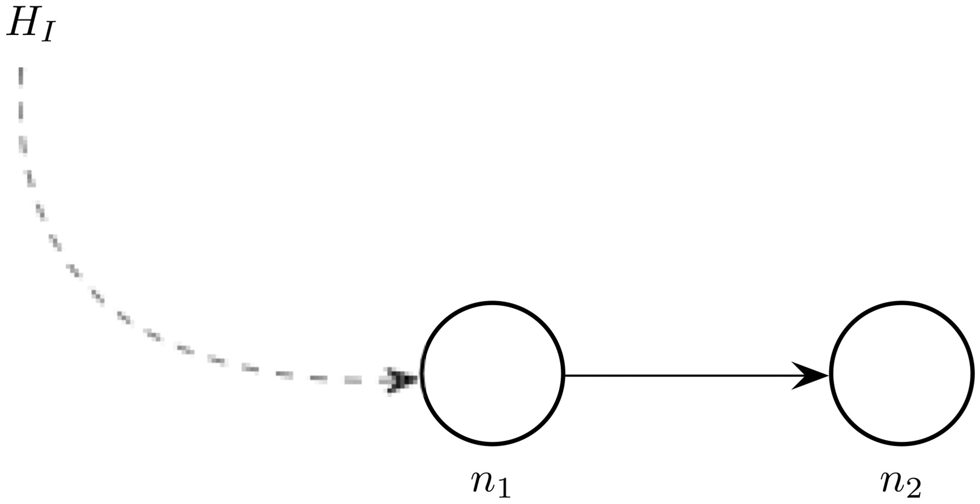
Due to the columnar representation, we identify the fiber F with the set \(S^\) of the preferred directions of the cells in the plane. Moreover, as it is represented in Fig. 1, cells with similar preferred directions are organized in columns perpendicular to the cortical surface. Directional columns are in turn grouped into hypercolumns (see Fig. 2), each of them coding for the full range of reaching directions.

Here we choose as a basis of the fiber bundle the cortical tuning of the position of the plane. Hence \(M\subset \mathbb ^\). There is wide neural literature supporting that M1 neurons encode hand positions (see e.g. Georgopoulos et al., 1984; Kettner et al., 1988; Schwartz, 2007, as well as Sections 2.1 and 2.2), but the way  how these positions are mapped on the cortical plane is not well understood. Possibly the position of the hand will be indirectly coded through the command to the specific group of muscles which will implement the movement (Schwartz et al., 1988; Georgopoulos, 1988). In particular, according to Graziano and Aflalo (2007) (see also Graziano et al., 2002; Aflalo & Graziano, 2006b; Graziano, 2008) the topographic organization in motor cortex emerge from a competition among three mappings: somatotopic map of the body; a map of hand location in space; a map of movements organization. Since these maps preserve a principle of local similarity, and we are considering here very simple hand movements, a fiber bundle structure in the position-directions is not inconsistent with these data. On the other side, from a functional point of view, it is clear that at every point of the 2D space the hand can move in any direction, and this aspect is captured by a fiber bundle of direction on a 2D spatial bundle.

E is the total tuning space to which motor cortical cells are selective and it is locally described by the product \(\mathbb ^\times S^1\);

\(\pi : E\rightarrow M\) is a projection on the \(\left( x,y\right)\) variables which acts as \(\pi \left( x,y,\theta \right) = \left( x,y\right)\).

A section \(\sigma : M\rightarrow E\) represents the selection of a point on a fiber of possible movement directions at position \(\left( x,y\right) \in M\), namely, it associates the point \(\left( x,y\right)\) to a point \(\left( x,y,\theta \right) = \sigma \left( x,y\right)\). A fiber \(E_= \pi ^\simeq S^\) corresponds to an entire hypercolumn. A schematic representation of the fiber bundle structure is shown in the right side of Fig. 6.

We recall that formula (2), which is equivalent of (6) for every fixed instant of time, selects the maximum of the scalar product in the direction of the trajectory of movement. This is equivalent to say that the spike probability is maximized if the scalar product in the direction orthogonal to that of motion vanishes. For our model it will be essential to consider this and to do so we will make use of the following definition. We call 1-form a function \(\omega = a_1 dx + a_2 dy\) which acts on a vector v as a scalar product:

$$\begin \omega (v) = \langle a, v \rangle . \end$$

(10)

In our case, to be compatible with Eq. (6), we will choose \(a= v^\perp\), where \(v= \left( \cos \theta , \sin \theta \right)\) denotes cell’s preferred movement direction. As a result \(a=(-\sin (\theta ), \cos (\theta ))\) and

$$\begin \omega = -\sin \theta \;\textrmx + \cos \theta \;\textrmy. \end$$

(11)

Fig. 6

(Left) In the up, motor cortical map of preferred directions referred to movements on a two-dimensional space (adapted from Naselaris et al., 2006). Colors denote preferred directions within the interval \(\left[ 0,2\pi \right]\). A conventional zoom and a superimposition of the lattice model (see Fig. 2) have been made in order to visualize the directional map referred to the size of the hypercolumns. (Right) Arm area of M1 modelled as a set of hypercolumns. Here, the angle \(\theta\) lies in the interval \(\left[ 0, 2\pi \right]\) and it is represented as an arrow

3.1.1 Neuronal population vector and distance

As we clarified, we are interested in the set of vectors on which the 1-form (11) vanishes. This set identifies a two-dimensional subset of the tangent space at every point, called horizontal distribution (see Definition 2). It can be represented as

$$\begin D_= \}_1 + \alpha _2 }_2: \alpha _1, \alpha _2\in \mathbb \}, \end$$

(12)

where the generators are

$$\begin }_1= \left( \cos \theta , \sin \theta , 0\right) \quad , \quad }_2= \left( 0, 0, 1\right) . \end$$

(13)

In terms of vector fields, they will be denoted respectively

$$\begin X_1= \cos \theta \frac + \sin \theta \frac\quad , \quad X_2= \frac. \end$$

(14)

According to Chow’s Theorem (see Montgomery (2006) and Agrachev et al. (2019) for a detailed analysis), vector fields (14) induce on the space \(\mathbb ^2\times S^1\) a distance d in terms of Definition 9.

We saw in Section 2.1 (see also Georgopoulos et al., 1986; Georgopoulos, 1988; Georgopoulos et al., 1988) that one estimate concerning the output of a population of M1 cells is given by the neuronal population vector (3). Its formula describes an expectation value weighted by the w-functions with respect to all possible cells preferred directions \(\theta '\in S^\). Basically each cell assigns a contribution to the output given by its own preferred direction modulated by the distance between the actual direction of movement and cell’s preferred direction itself. As reported in Naselaris et al. (2006), within each hypercolumn the neuronal population vector ensures a good estimate of a reaching direction. These results suggest that within each hypercolumn of M1 there is a local and isotropic activity pattern characterized by the weight functions. We observe that the weight (4) can locally be approximated through Taylor expansion by

$$\begin \cos (\theta - \theta ') \simeq 1 - \frac \simeq e^}. \end$$

Since for small values of \(\theta\) the distance in the circumference is \(\left| \theta - \theta '\right|\), this suggests approximating the discrete formula (3) with the continuous correspective in which the weight (4) is replaced with the exponential

$$\begin P\left( \theta \right) = \int _0^ e^ e^} d \theta '. \end$$

(15)

This formula can also be exploited in our case. Indeed, if we denote by d the distance induced by vector fields \(X_1\) and \(X_2\) (see Definition 9), we can provide an estimate of the collective behaviour of cells tuning with respect to a selective point \(\left( x,y,\theta \right)\) within a hypercolumn of positions and directions of movement:

$$\begin P\left( x,y,\theta \right) := \int _\int _^ g_\left( x',y', \theta '\right) \omega \left( \left( x,y,\theta \right) , \left( x',y',\theta '\right) \right) dx'dy'd\theta ', \end$$

(16)

where \(D\subset \mathbb ^2\) is a subset of a cortical module and the function \(\left( x',y', \theta '\right) \mapsto g_\left( x',y', \theta '\right)\) represents the single cell’s spike probability density in response to \(\left( x,y,\theta \right)\):

$$\begin g_\left( x',y', \theta '\right) = e^. \end$$

(17)

The above equation is the analogue of Hatsopoulos model (7) only in relation to the variables of position and direction of movement. The new weighting function

$$\begin \omega \left( \left( x,y,\theta \right) , \left( x',y',\theta '\right) \right) = e^} \end$$

(18)

measures the closeness between the cellular selectivity of the points \(\left( x,y,\theta \right)\) and \(\left( x',y',\theta '\right)\). Therefore, formula (18) is intended to express a core of connectivity (local, since it is evaluated in a small cortical module) that is functional. We will see that the analogous for this area of formula (18) is provided by Bressloff and Cowan (2003) and Sarti and Citti (2015) models in the visual cortex.

3.1.2 Comparison of the static model with primary visual cortex V1

An analogy on the selectivity behaviour of external features with neurons in the primary visual cortex area (V1) is evident. (Hubel & Wiesel, 1977; Hubel, 1995) discovered that to every retinal position is associated an hypercolumn of cells sensible to all possible orientations. A simplified representation is shown in the right side of Fig. 7. Since the early ‘70s, a large number of differential models were developed for visual cortex areas, starting with Hoffman (1970), Petitot and Tondut (1999), Bressloff and Cowan (2003), Citti and Sarti (2006), just to name a few of the main ones. Their models describe the functional architecture of V1 trough geometric frameworks such as contact bundles, jet bundles or Lie groups endowed with a sub-Riemannian metric.

Fig. 7

(Left) Layout of orientation preferences in the visual cortex. At singular points (pinwheels), all orientations meet. Source: Bosking et al. (1997). (Right) V1 modelled as a set of hypercolumns

In particular, the model expressed through the one-form (11) matches the one proposed by Citti-Sarti in 2006 (Citti & Sarti, 2006) for the description of image edge selectivity by V1 cells. Both for V1 and the arm area of M1, the total space of the fiber bundle is three-dimensional, whereas the cortical layers are of dimension two, so that a dimensional constraint has to be taken into account. In Fig. 7, the orientation preferences of simple cells in V1 are color coded and every hypercolumn is represented by a pinwheel (see the work of Petitot (2003) neurogeometry}). For the motor cortex, a “directional map” is suggested from Fig. 2, for which PDs are repeatedly arranged on the motor cortical layer in such a way that, within a given locale (hypercolumn), the full range of movement directions are represented. Moreover, as distance increases away from the center of the hypercolumn (black filled circle), up to the radius of the hypercolumn (120 \(\mu\)m), PDs diverge from that at the center of the circle (see Figs. 7 and 6 for a direct comparison). We add that cells preferred directions in M1 are correlated across very small distances along the tangential dimension (see Amirikian & Georgopoulos, 2003) and this type of arrangement is consistent with the smooth variation of orientation preference observed in V1 (see Hubel & Wiesel, 1963). Moreover, the radii of the hypercolumns of arm area M1 and V1 are of the same order size and are respectively of 240 and 200\(\mu\)m.

One of the greatest difficulties and differences in modelling the functional architecture of M1 is the absence of an analogue of the simple cells receptive profiles, which we might call “actuator profiles". Simple cells of visual areas are indeed identified by their receptive field (RF) which is the domain, subset of the retinal plane, to which each cell is sensible in response to a visual stimulus. Activation of a cell’s RF evokes the impulse response, which is called the receptive profile (RP) of the cell. A widely used model (Jones, 1987; Daugman, 1985; Lee, 1996) for the RP representation of a simple cell located at the retinal position q and selective to the feature p, is in terms of Gabor filters \(\psi _: \mathbb ^2\rightarrow \mathbb \),

$$\begin \psi _\left( x\right) = e^e^. \end$$

(19)

Although it is not well understood the presence or the definition of such functions for M1, we argue that the action of primary motor cortical cells occurs in a comparable way as in V1. This hypothesis is primarily supported by the tuning functions (2) and (5) expressed by Georgopoulos (see 2.1 and Georgopoulos et al. 1982; Schwartz et al. 1988) and through the trajectory encoding model (7) provided by Hatsopoulos (see 2.2 and Hatsopoulos et al., 2007). Their models share the selective tuning of neurons by evaluating the alignment between an external input variable and the individual cell’s preferred feature via a scalar product. Analogously for V1, the linear term in (19) evaluates the aligning between cell’s selective feature p with respect to the input x. Bressloff and Cowan (2003) (see also Bressloff et al., 2002; Wilson & Cowan, 1973) proposed to represent the stationary state of a population of simple cells through equation

$$\begin a\left( \phi ,r\right) =& \frac\int _^ \omega _}\left( \phi , \phi '\right) \sigma \left( a\left( \phi ,r\right) \right) \textrm\phi '+ \frac\int _}\omega _}\left( s\right) \sigma \left( a\left( \phi ,r+ se_\right) \right) \textrms, \end$$

(20)

where \(\omega _}\) and \(\omega _}\) correspond to the strength of connections from the iso-orientation patch within and between the hypercolumns of V1, respectively. The function \(a\left( \phi ,r\right)\) is the activity in an iso-orientation patch at the point r with orientation preference \(\phi\), whereas \(\sigma \left( a\right)\) is a smooth sigmoidal function of the activity a and \(\alpha\), \(\mu\) are time and coupling constants. The weight \(\omega _}\) represents the isotropic pattern of activity within any one hypercolumn, and in Bressloff and Cowan (2003), in the simplified case where the spatial frequencies are not taken into account, it is modelled by

$$\begin \omega _}^\left( \phi \right) = \frac\left( \cos \left( \phi - \phi '\right) + \cos \left( \phi +\phi '\right) \right) , \quad \phi ,\phi '\in S^1. \end$$

(21)

Equation (21) is the analogous of the weighting function (4) assumed by Georgopoulos. In the work of Sarti and Citti (2015) both contributions of \(\omega _\) and \(\omega _\) are modelled by means of a single connectivity kernel given by

$$\begin \omega \left( \left( \phi , r\right) , \left( \phi ', r'\right) \right) = e^,\quad \left( \phi , r\right) , \left( \phi ', r'\right) \in SE\left( 2\right) , \end$$

(22)

where \(d_c\) is a Carnot Carathéodory distance associated to the cortical feature space identified with the special Euclidean group \(SE\left( 2\right) \simeq \mathbb ^2\times S^1\). We will see in a higher dimensional model that a connectivity kernel of this type can be used to interpret the segmentation of neural activity in neural states (Section 5).

3.2 A 2D kinematic tuning model of movement directions

Now we aim at realizing a unified neurogeometrical framework that generalizes the preceding model of movement fiber bundle structures.

We will describe a sub-Riemannian model such that motor cortical cells selective behaviour can be represented through integral curves of the cortical features space of time, position, direction of movement, speed and acceleration. The resulting model will present time dependent variables, which seems particularly natural for a model of movement.

3.2.1 Integral curves and time dependent PD

We represent motor cortical cell tuning variables by the triple \(\left( t, x, y\right) \in \mathbb ^3\), which accounts for a specific hand’s position in time. We also consider the variable \(\theta \in S^1\) which encodes hand’s movement direction, and the variables v and a which represent hand’s speed and acceleration along \(\theta\). The triple \(\left( t, x, y\right) \in \mathbb ^3\) is assumed to belong to the base space of the new fiber bundle structure, whereas the variables \(\left( \theta , v, a\right) \in S^1 \times \mathbb ^\) form the selected features on the fiber over the point \(\left( t, x, y\right)\). We therefore consider the 6D features set

$$\begin \mathcal = \mathbb ^_ \times S^1_ \times \mathbb ^_, \end$$

(23)

where this time the couple \(\left( x,y\right) \in \mathbb ^2\) represents the cortical tuning for hand’s position in a two dimensional space.

We refer to Eq. (7) to recall that the spike probability of a neuron is maximized in the direction of the movement fragment. Therefore, as in Section 3.1, the choice of the variables with their differential constraints induce the vanishing of the following 1-forms

$$\begin \omega _= \cos \theta \textrmx + \sin \theta \textrmy - v\textrmt= 0,\quad \omega _ = -\sin \theta \textrmx + \cos \theta \textrmy= 0, \quad \omega _ = \textrmv -a\textrmt= 0. \end$$

(24)

The one-form \(\omega _\) encodes the direction of velocity over time: the unitary vector \(\left( \cos \theta , \sin \theta \right)\) is the vector in the direction of velocity, and its product with \(\left( \dot, \dot\right)\) yields the speed. As we already noted, conditions above are equivalent to find vector fields orthogonal to \(\omega _i\). Consequently, the associated horizontal distribution \(D^}\) turns out to be spanned by the vector fields

$$\begin X_= v\cos \theta \frac} + v\sin \theta \frac}+ a\frac}+ \frac},\quad X_= \frac},\quad X_= \frac}. \end$$

(25)

Note that, if we prescribe time, movement direction and acceleration, we can deduce by integration first speed and then location. This is the reason why we prescribe only these 3 vector fields: \(X_1\) prescribes the change in time, \(X_2\) in the direction of movement and \(X_3\) in the acceleration. In addition, not all curves are physically meaningful in this space: it is not possible for a curve to change its velocity \(v=v(t)\) while the position (x, y) remains constant. Hence we have to restrict the set of admissible curves and define horizontal ones. Horizontal curves of the space are integral curves of the vector fields \(X_1, X_2\) and \(X_3\) and are of the form

$$\begin \gamma '\left( s\right) = \alpha _1\left( s\right) X_\left( \gamma \left( s\right) \right) + \alpha _2\left( s\right) X_\left( \gamma \left( s\right) \right) + \alpha _3\left( s\right) X_\left( \gamma \left( s\right) \right) , \end$$

(26)

where the coefficients \(\alpha _i\) are not necessarily constants.

We recalled in Section 2.2 that M1 cells are not selective to a single movement direction, but the preferred movement direction varies in time (Churchland & Shenoy, 2007; Hatsopoulos et al., 2007). In particular, in Fig. 3b we reproduced data from Churchland and Shenoy (2007), where the PD of a single M1 neuron was represented as a curve dependent on time.

We propose the curves expressed in (26) as a model of the integrated selective behaviour of M1 neurons. Note in particular that the t component of the horizontal curve \(\gamma\) satisfies \(t' = \alpha _1\). This means that the coefficient \(\alpha _1\) is a modulation of the time, and can account for the difference between the external time and the perceived one. By simplicity, we will assume that the two times coincide, therefore we will assume \(\alpha _1=1\) from now on. In the sequel we will see that it is possible to choose coefficients in Eq. (26) which allow to recover the full fan of curves reproduced in Fig. 3. The expression of \(\dot\) described in (40) is the coefficient of the vector field \(X_2\) and the expression of \(\dot\) described in (41) is the coefficient of the vector field \(X_3\):

$$\begin \dot\left( t\right) = X_\left( \gamma \left( t\right) \right) + \dot\left( t\right) X_\left( \gamma \left( t\right) \right) + \dot\left( t\right) X_\left( \gamma \left( t\right) \right) . \end$$

(27)

The functions \(t\mapsto \dot\left( t\right)\) and \(t\mapsto \dot\left( t\right)\) represent, respectively, the rate of change of the selective tuning to movement direction and acceleration variables.

3.2.2 Time-dependent neuronal population vector

By analyzing the following commutation relations

$$\begin \left[ X_, X_\right] = v\sin \theta \frac}&- v\cos \theta \frac}=: X_,\quad \quad \left[ X_, X_\right] = \frac}=: X_,\\&\left[ X_, X_\right] = \cos \theta \frac}+ \sin \theta \frac}=: X_, \end$$

(28)

we observe that \(\left( X_i\right) _^\) are linearly independent. Therefore, all \(\left( X_i\right) _^\) belonging to \(D^}\) together with their commutators span the whole tangent space at every point, meaning that Hörmander condition is fulfilled (see Appendix A for a brief review). Thanks to Hörmander condition, it is possible to define a metric \(d_}\) in the cortical feature space \(\mathcal \). This allow to formally consider the analogous of the population vector (16) defined in Section 3.1.1 (see as well Definition 9). Indeed, we will call as time dependent neural population vector an estimate of the collective behaviour of cells tuning around a cortical module centered at point \(\eta _0\in \mathcal \). We define it by means of the following

$$\begin P_}\left( \eta _0\right) := \int _h_\left( \eta \right) \omega _}\left( \eta _0,\eta \right) \textrm\eta , \end$$

(29)

where \(E\subset \mathcal \) is a neighbourhood of \(\eta _0\) and the weighting function

$$\begin \omega _}\left( \eta _0,\eta \right) = e^}\left( \eta _0,\eta \right) ^2} \end$$

(30)

encodes an estimate of the local connectivity between the cortical tuning points \(\eta _0\) and \(\eta\). The function \(\eta \mapsto h_\left( \eta \right)\) corresponds to the contribution provided by the variable \(\eta\) in the population coding. As in Hatsopoulos model (7), it is the spike probability of a neuron in response to the input variable \(\eta _0\):

$$\begin h_\left( \eta \right) = e^. \end$$

(31)

The definition of (30) embodies the same meaning as the weighting function (18) showed in the “static" model and in the models for visual areas (see Eqs. (21) and (22) in Sect. 3.1.2 defined in Bressloff & Cowan, 2003; Sarti & Citti, 2015). It represents the local interactions between cells within a cortical module by means of a distance of the cortical feature space.

Due to the works of Nagel et al. (1985) and Montgomery (2006), it is possible to provide a local approximation of distance \(d_}\) in terms of a homogeneous distance (see Definition 10), as follows

$$\begin d_}\left( \eta _0,\eta \right) \simeq \left( \left| c_1 e_\right| ^ + \left| c_2e_\right| ^+ \left| c_3e_\right| ^+ \left| c_4e_\right| ^3+ \left| c_5e_\right| ^3+ \left| c_6e_\right| ^2 \right) ^}, \end$$

(32)

where \(\left( \eta _0,\eta \right) = \left( \left( t_0,x_0,y_0,\theta _0, v_0, a_0, \right) ,\left( t, x,y,\theta , v, a, \right) \right) \in \mathcal ^2\), \(c_i\) are non negative constant coefficients, th