
記住我


In its simplest form, geometric singular perturbation theory assumes that a general model is defined in terms of an explicit fast-slow decomposition of the form
$$\begin \left\ x^ = f(x, y, \epsilon ), \\ y^ = \epsilon \, g(x, y, \epsilon ), \end \right. \end$$
(1)
where \(0 < \epsilon \ll 1\) is a small parameter, so that the fast variable is \(x \in \mathbb ^m\) and the slow variable is \(y \in \mathbb ^n\). In the limit \(\epsilon \rightarrow 0\), system (1) reduces to a lower-dimensional, so-called fast subsystem
$$\begin x' = f(x, y, 0), \end$$
(2)
where the slow variable y plays the role of a constant parameter vector. The equilibria of the fast subsystem (2) form a manifold \(\mathcal \) in (x, y)-space,
$$\begin \mathcal = \^m \times \mathbb ^n \; \mid \; f(x, y, 0) = 0 \}, \end$$
which is called the critical manifold of system (1). We assume that \(\mathcal \) is Z-shaped with respect to the component of x that represents voltage v. This means that \(\mathcal \) has (at least) three co-existing equilibrium branches, parameterized by y. Ordered with respect to their corresponding v-components, we refer to these branches as the lower (silent) branch, the middle branch, and the upper (active) branch of \(\mathcal \).
For both SW and PP bursting, certain additional features must be present: firstly, that system (2) has a (lower) saddle-node bifurcation at some critical parameter value \(y_\textsf\), at which the lower and middle branches of \(\mathcal \) meet; and secondly, that system (2) has an Andronov–Hopf bifurcation along the upper branch of \(\mathcal \), which gives rise to a family \(\mathcal \) of periodic orbits of (2) parameterized by y. Note that this second requirement implies \(m \ge 2\); that is, the fast variable x must be at least two dimensional. Crucially, this Andronov–Hopf bifurcation is subcritical in the PP case, which means that the orbits of \(\mathcal \) are unstable and, hence, system (2) does not produce stable spiking activity for initial conditions along the upper (active) branch of \(\mathcal \). For SW bursting, on the other hand, there exists a stable family of periodic orbits, together with a mechanism that induces a transition from the active phase to the silent phase. The originally described and most commonly considered form of SW bursting involves a supercritical Andronov–Hopf bifurcation for (2) on the upper (active) branch of \(\mathcal \) and a homoclinic bifurcation at which the family \(\mathcal \) of stable periodic orbits collides with a saddle equilibrium on the middle branch of \(\mathcal \) (Rinzel, 1986).
While the presence and order of specific bifurcations in the fast subsystem (2) help to predict the burst pattern exhibited by the full model, the burst pattern also depends on the relative location of the nullcline associated with the slow variable. In order for models to exhibit SW bursting, for example, it is necessary, although not sufficient, for the slow nullcline to intersect the middle branch of \(\mathcal \) at an equilibrium point below the homoclinic bifurcation; in particular, the full system must have a steady state that is of saddle type. We make sure this is the case over a sufficiently large range of parameters for all models considered in this paper.
2.1 Models and parameter-dependence of bursting dynamicsAs mentioned in the introduction, we select and study four different, low-dimensional SW bursting models with distinct formulations of the fast inward current. Each is presented in this section in its original form, and we discuss the parameter range for the maximal conductance of the fast inward current, \(g_\) or \(g_\), over which SW bursting occurs.
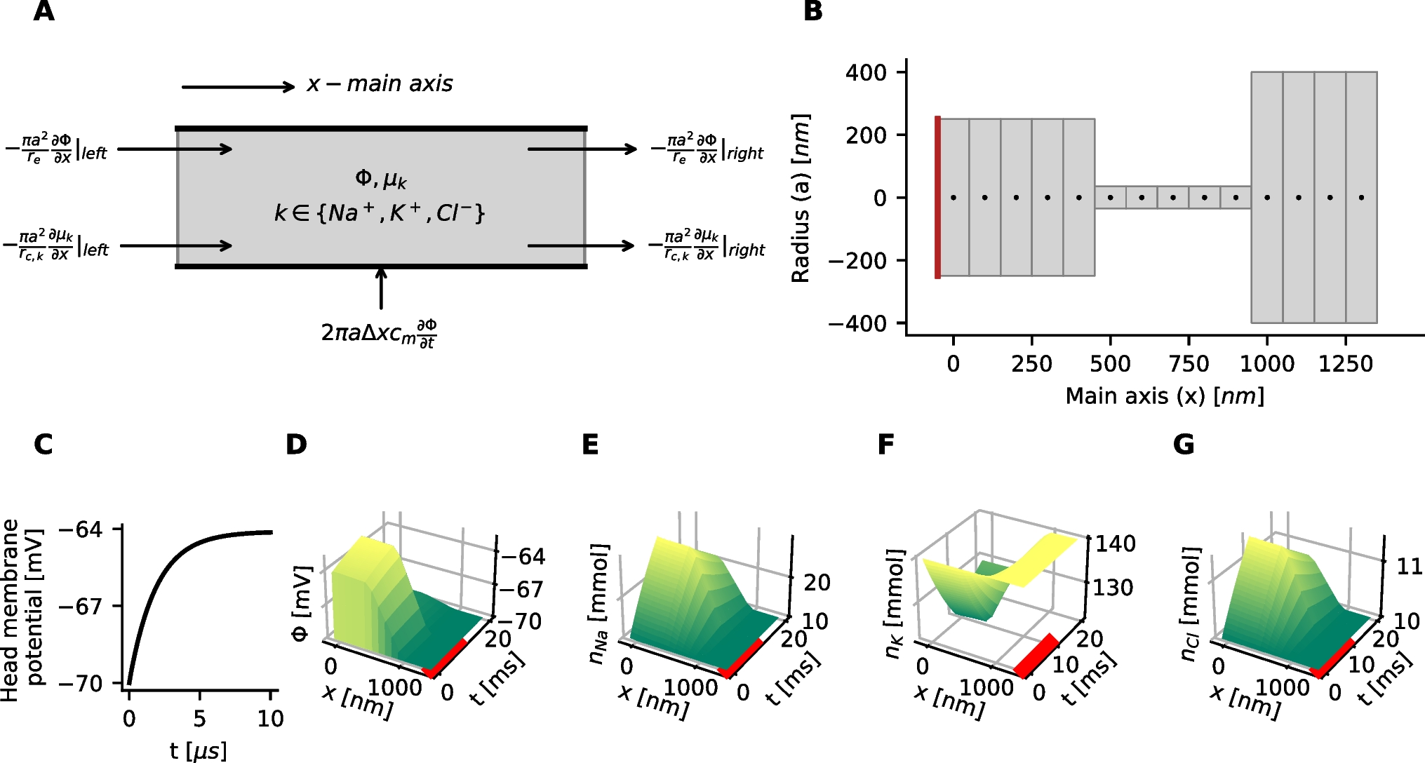
2.1.1 Generic endocrine modelTsaneva-Atanasova et al. (2010) introduced a generic endocrine model that exhibits both SW and PP bursting over physiologically relevant parameter ranges. The model is a system of differential equations for the membrane potential v, the gating variable n of the K\(^+\) channel, and the calcium concentration c in the cytosol. The equations take the form
$$\left\ c_mv'&=-I_(v)-I_K(v,n)-I_(v,c),\\ n'&=(n_\infty (v)-n)/\tau _n,\\ c'&=-f_c(\alpha I_(v)+k_pc)\end\right.$$
(3)
for constants \(c_m\), \(\tau _n\), \(f_c\), \(\alpha\), and \(k_p\). The expressions for the currents and steady state activation functions are given by:
$$\begin I_(v) &= g_ \, m_^2(v) \, (v - e_), \\ I_K(v,n) &= g_ \, n \, (v - e_),\\ I_(v,c) &= g_ \, \left( \dfrac \right) \, (v - e_), \\ m_(v) &= (1 + e^)^, \\ n_(v) &= (1 + e^)^. \end$$
(4)
We choose default parameter values as given in Table 1, for which the model exhibits the SW bursting pattern shown in Fig. 2A. Indeed, non-dimensionalization (see the Appendix) shows that the three-dimensional system (3) and (4) readily separates into fast and slow equations, because v changes at a rate \(R_v \approx 716\) that is faster than the rate \(R_n \approx 33\) for n which, in turn, is significantly faster than the rate \(R_c \approx 1.7\) for c. We consider v and n as two fast variables and c as one slow variable, so that system (3) and (4) has the lowest possible dimensions for SW bursting; the alternative pairing of one fast and two slow variables would be relevant for studying canard dynamics (Vo et al., 2013), but we do not consider this here. More details about the model can also be found in (Tsaneva-Atanasova et al., 2010).
Fig. 2
Fast-slow decomposition for the generic endocrine model (3) and (4). A SW bursting for default parameter values given in Table 1. B Bifurcation diagram of the model’s fast subsystem with respect to the slow variable c, with bifurcation points labeled and the burst trajectory, which evolves clockwise, overlaid in gray. Oscillations start after the trajectory jumps up from the lower left saddle node (LSN) and stop when it reaches the homoclinic (HC). C The model exhibits PP bursting when \(g_\) is increased to 1.5; note that the ranges of c in (A) and (C) are different. D Bifurcation diagram as in (C) but with \(g_ = 1.5\); the PP burst trajectory, which also evolves clockwise, is again overlaid in gray. The labels SupAH (B) and SubAH (D) refer to supercritical and subcritical Andronov–Hopf bifurcations, respectively
Table 1 Generic Endocrine Model (3) and (4): default parameter valuesThe fast subsystem, consisting of the (v, n)-equations in (3) and (4), and its attractors can be studied by considering the slow variable c as a bifurcation parameter. The corresponding bifurcation diagram, shown in Fig. 2B, forms a scaffold for understanding the burst pattern that the full model produces. Specifically, based on this fast-slow decomposition, we can assume that any general initial position with slow variable \(c = c_0\) lies on a trajectory that predominantly evolves under the fast dynamics to one of the attractors that exists in the fast subsystem for \(c = c_0\). Subsequently, the sign of \(c'\) will determine whether the trajectory drifts to the left or right along the corresponding attractor branch until either this branch terminates and a transition to a new attractor occurs, the trajectory goes off to infinity, or a stable state for the full system is reached. In Fig. 2B, for (3) and (4) with default parameter values, the c-nullcline (dashed curve) cuts through the middle branch of the critical manifold \(\mathcal \), just below HC in the bifurcation diagram. According to the equation for c in (3) and (4), we have \(c' < 0\) below this nullcline. Hence, c is decreasing during the silent phase and, as suggested by the bifurcation diagram of the fast subsystem, the active phase of the SW burst starts due to a jump up in potential v from the c-value at which the fast subsystem undergoes a saddle-node bifurcation (LSN). For this c-value, the attractor of the fast subsystem at elevated voltage is a periodic orbit, part of a family of such orbits that originates in a supercritical Andronov–Hopf bifurcation (SupAH). Thus, oscillations result, and they continue as c increases, according to its equation in (3) and (4), until a homoclinic bifurcation (HC) occurs. At that bifurcation, the trajectory returns to the silent phase, where it is attracted to the stable equilibria on the lower (silent) branch of \(\mathcal \).
When \(g_\) is increased from its default value of 0.81 to \(g_ = 1.5\), the model exhibits the qualitatively different PP bursting pattern (Fig. 2C). The bifurcation diagram of the fast subsystem with respect to the variable c has changed correspondingly (Fig. 2D). In particular, we see that the Andronov–Hopf bifurcation point has now moved to a larger c-value and has changed criticality to become subcritical (SubAH). Therefore, the fast subsystem now has a family of unstable periodic orbits. Hence, after the jump up from LSN, the trajectory is attracted to the upper branch of the critical manifold \(\mathcal \), which comprises stable equilibria of the fast subsystem. Since these equilibria are foci, the trajectory spirals around the upper branch of \(\mathcal \) while slowly moving to the right with respect to c. This behavior generates a voltage plateau in the active phase, accompanied by rapidly decaying oscillations in lieu of spikes (Fig. 2C). The upper branch of \(\mathcal \) loses stability at SubAH, and after a small delay associated with the slow passage through an Andronov–Hopf bifurcation (Baer et al., 1989; Baer & Gaekel, 2008; Neishtadt, 1987, 1988), the trajectory jumps down to the silent phase where it flows back to LSN to complete a burst cycle.
The bifurcation diagrams in Fig. 2 display SW and PP bursting patterns produced by the generic endocrine model (3) and (4) for two fixed values of \(g_\). The robustness of these patterns and the transition between them can be studied more systematically by considering a two-parameter bifurcation diagram. Specifically, we can follow the codimension-one bifurcations labeled LSN, USN, SupAH, SubAH and HC in Fig. 2B, D as curves in the two-parameter \((c, g_)\)-plane. The resulting bifurcation diagram is displayed in Fig. 3A.
Fig. 3
Dependence on \(g_\) of bifurcation curves for the fast subsystem of the generic endocrine model (3) and (4). A Two-parameter bifurcation diagram in the \((c, g_)\)-plane. The locus AH of Andronov–Hopf bifurcations (blue) comprises the two curves SupAH and SubAH that meet at the generalized Hopf point labeled GH (left black star); SupAH and the curve HC of homoclinic bifurcations merge and end at a Bogdanov–Takens point (BT; right black star) on the curve USN of saddle-node bifurcations (red). The SW and PP bursting regions are shaded red and blue, respectively. The black dashed lines correspond to the examples of SW bursting for \(g_=0.81\) and PP bursting for \(g_=1.5\) shown in Fig. 2. B Lyapunov coefficent along the curve AH. The Andronov–Hopf bifurcation is supercritical until this coefficient increases through 0 for \(g_\) just below 1, corresponding to the point GH, and subcritical for \(g_\)-values above that
The two-parameter bifurcation diagram shows how the bifurcation points change, and in some cases meet and disappear, when \(g_\) varies away from its default value of 0.81 (bottom dashed line). In particular, the curves SupAH (light blue) and HC (green) of supercritical Andronov–Hopf and homoclinc bifurcations, respectively, end on the curve USN of saddle-node bifucation (red) at the codimension-two Bogdanov–Takens point BT (right black star). Furthermore, the curve SupAH transitions to SubAH by changing criticality at the generalized Hopf point GH (black star just below \(g_ = 1\) on the curve AH in the diagram), which occurs when the first Lyapunov coefficient associated with the Andronov–Hopf bifurcation changes sign (Fig. 3B); this first Lyapunov coefficient was computed numerically with MATCONT (Dhooge et al., 2003). The curve subAH (dark blue) of subcritical Andronov–Hopf bifurcations then moves into the V-shaped region between the two curves LSN and USN. At the point GH, a curve of saddle-node bifurcation of periodic orbits (SNPO) originates and progresses to larger c-values as \(g_\) continues to increase, until it ends just above \(g_ = 1.5\) on the curve HC. In the remainder of the paper, we will denote as AH the locus or curve of Andronov-Hopf bifurcation comprised of the components SupAH and SubAH.
The lower black dashed line in Fig. 3A corresponds to the bifurcation diagram for \(g_ = 0.81\) in Fig. 2B that gives rise to SW bursting. In the direction of increasing c, we successively encounter the supercritical Andronov–Hopf bifurcation SupAH (light blue), the saddle-node bifurcation LSN (red), the homoclinic bifurcation HC (green), and the other saddle-node bifurcation USN (red). If we use \(c_\textsf\) to denote the c-value at which a bifurcation of type \(\textsf\) occurs, then the order of bifurcations for fixed \(g_ = 0.81\) is \(c_\textsf< c_\textsf< c_\textsf< c_\textsf\). This order of bifurcations is maintained for lower values of \(g_\), until HC disappears, just below the point BT. Hence, since \(c_\textsf < c_\textsf\), the active phase is characterized by stable periodic orbits, and persists until \(c \approx c_\textsf\); we conclude that these \(g_\)-values all give rise to SW bursting. Similarly, for larger \(g_\)-values, even though SubAH and LSN cross, the change in criticality at GH implies that the active phase is still characterized by stable periodic orbits until the saddle-node bifurcation of periodic orbits SNPO occurs after LSN; that is, for SW bursting, we require \(c_\textsf < c_\textsf\).
The order of the bifurcations along the black dashed line for \(g_ = 1.5\) in Fig. 3A, which corresponds to PP bursting shown in Fig. 2D, is \(c_\textsf< c_\textsf< c_\textsf< c_\textsf < c_\textsf\); it is important that \(c_\textsf\) is only just smaller than \(c_\textsf\), which means that this order generates a PP pattern that is qualitatively similar to that for \(g_\)-values above the point where SNPO ends, which feature the bifurcation sequence \(c_\textsf< c_\textsf< c_\textsf < c_\textsf\). While we did not check all \(g_\)-values, this order of bifurcations is maintained until at least \(g_ = 2\).
The red and blue shaded regions in Fig. 3A show the ranges of \(g_\)-values over which the generic endocrine model (3) and (4) can potentially exhibit SW and PP bursting, respectively. Choosing parameters in one of these regions is, in fact, not sufficient to ensure that the corresponding burst pattern occurs, since the actual burst pattern also depends on the position of the c-nullcline — which changes with \(g_\) due to the presence of \(I_\) in the c-equation in (3) and (4) — and the speed at which c evolves. We conclude from this diagram, however, that SW bursting can at most be maintained for \(0.65< g_ < 1.1\).
Figure 4 compares the burst patterns of the generic endocrine model (3) and (4) for different values of \(g_\). At \(g_ = 0.75\), the model exhibits SW bursting (Fig. 4A) that is very similar to that for the default value \(g_ = 0.81\) (Fig. 2A). When \(g_\) is increased to 1.0, the model still exhibits SW bursting (Fig. 4B), but the increase in \(g_\) strengthens \(I_\), which results in more elevated v values at peaks of the bursts. At this elevated v, the current \(I_K\) activates more strongly compared to the previous case, resulting in stronger hyperpolarizations between spikes and fewer spikes in the burst. When \(g_\) is increased still further to 1.6, the activity pattern transitions to PP bursting (Fig. 4C). This case yields the strongest \(I_\) activation of the three; indeed, despite the induced elevation of v and corresponding strong activation of \(I_K\), the latter current cannot overcome \(I_\) and cause repolarization. Thus, the equilibria on the upper branch of the critical manifold \(\mathcal \) stabilize and spike oscillations during the active phase are prevented.
Fig. 4
Burst patterns exhibited by the generic endocrine model (3) and (4) for different values of \(g_\), along with associated currents. A SW bursting at \(g_=0.75\). B SW bursting at \(g_=1.0\) with larger amplitude spikes than in (A). C PP bursting for \(g_ = 1.6\)
2.1.2 Sodium-potassium minimal modelThe sodium-potassium minimal model introduced in (Izhikevich, 2007) is an example of an SW burster comprised of only the basic essentials needed to burst. This model consists of the following differential equations:
$$\left\ c_m \, v' & = -I_L(v) - I_(v) - I_K(v,n) - I_(v,s) + I, \\ n' &= (n_(v) - n)/\tau _n, \\ s' &= (s_(v) - s)/\tau _s. \end \right.$$
(5)
The expressions for the currents and steady state activation functions for the model are given by:
$$\begin I_(v) &= g_l \, (v - e_l), \\ I_(v) &= g_ \, m_(v) \, (v - e_), \\ I_K(v,n) &= g_ \, n \, (v - e_), \\ I_(v,s) &= g_ \, s \, (v - e_), \\ m_(v) &= (1 + e^)^, \\ n_(v) &= (1 + e^)^, \\ s_(v) &= (1 + e^)^. \end$$
(6)
Note that \(I_S\) denotes a potassium current with gating that evolves much slower than that for \(I_K\). Again, we choose default parameter values, given in Table 2, for which the model exhibits SW bursting as shown in Fig. 5A. The bifurcation diagram of the model’s fast subsystem for default parameter values is shown in Fig. 5B. Notice that the order of bifurcations, in the direction of increasing s, is the same as in Fig. 2B, that is, \(s_\textsf< s_\textsf< s_\textsf< s_\textsf\).
Fig. 5
Dynamics and bifurcation structure for the sodium-potassium minimal model (5) and (6). A SW bursting for the default parameters given in Table 2. B Bifurcation diagram of the model’s fast subsystem with respect to the slow variable s for default parameter values, with the SW burst overlaid in gray. C Two-parameter bifurcation diagram of the fast subsystem in the \((s, g_)\)-plane; colors are as in Fig. 3A and the SW bursting region is shaded red. For realistic values (\(s<1\)), this model does not transition to PP. The light-blue shaded region corresponds to \(g_\)-values for which the full system has a stable steady state at elevated v. D Lyapunov coefficient along the curve SupAH. The Andronov–Hopf bifurcation is supercritical until around \(g_=65\), which lies outside the range shown in panel (C)
Table 2 Sodium-Potassium Minimal Model (5)–(6): default parameter valuesBy comparing timescales after non-dimensionalization of this model (see the Appendix), we find that the timescale constants of v, n and s are approximately \(R_v \approx 20\), \(R_n \approx 6.57\) and \(R_s \approx 0.005\), respectively. The rate \(R_v \approx 20\) varies linearly with \(g_\) as long as \(g_ > 9 = g_k\); if \(g_\) is decreased below this value, \(R_v \approx 9\) is determined by \(g_k\) instead and any further decrease in \(g_\) would not affect \(R_v\). Hence, the variables v and n are considerably faster than s, irrespective of the value for \(g_\).
Even though the sodium-potassium minimal model (5) and (6) is designed to exhibit SW bursting, it is capable of other activity patterns. For example, Supplemental Fig. 1 shows the non-spiking pattern generated for \(g_ = 35\) in which all solutions are attracted to a stable steady state at an elevated voltage level, which corresponds to a state of depolarization block. For this large value of \(g_\), the nullcline of the slow variable s intersects the upper branch of the critical manifold, which gives rise to a stable steady state of the full system. However, SW bursting is already lost for smaller \(g_\)-values. Figure 5C shows the two-parameter bifurcation diagram of the fast subsystem in the \((s, g_)\)-plane. As in Section 2.1.1, the ordering of bifurcation curves suggests that system (5) and (6) can potentially exhibit SW bursting for \(g_\)-values between 20 and 25, if the slow dynamics is tuned appropriately; this region is again shaded red. We computed the first Lyapunov coefficient associated with the Andronov-Hopf bifurcation (Fig. 5D) and found that it is negative for the default \(g_\) and remains so up until a much larger value, \(g_ \approx 65\). Hence, this system does not transition to PP bursting, at least not for \(s \in (0,1)\), the physically relevant range. Instead, for \(g_ > 32\) or so, system (5) and (6) moves into a state of depolarization block, which is the region shaded light blue in Fig. 5B.
2.1.3 Minimal Chay-Keizer modelNext, we consider the minimal Chay–Keizer model described in (Rinzel, 1986; Rinzel & Lee, 1986). This model takes the form:
$$\begin \left\ c_m \, v^&= -I_(v) - I_(v) -I_K(v, n) - I_(v, c), \\ n^&= (n_(v) - n)/\tau _n(v), \\ c^&= -f_c \, (\alpha \, I_(v) \, + k_ \, c). \end \right. \end$$
(7)
The currents and steady state activation functions for the model are given by:
$$\begin I_L(v) &= g_l \, (v - e_l), \\ I_(v) &= g_ \, m_^3(v) \, h_(v) \, (v - e_), \\ I_K(v, n) &= g_ \, n \, (v - e_), \\ I_(v, c) &= g_\, } \, (v - e_), \\ a_m(v) &= }}, \\ b_m(v) &= 4 \, e^, \\ m_(v) &= }, \\ a_n(v) &= }}, \\ b_n(v) &= 0.125 \, e^, \\ n_(v)&= }, \\ \tau _n(v) &= }, \\ a_h(v) &= 0.07 \, e^, \\ b_h(v) &= + 1}}, \\ h_(v) &= }. \end$$
(8)
We choose the default parameter values given in Table 3, for which the model exhibits SW bursting as displayed in Fig. 6A.
Fig. 6
Dynamics and bifurcation structure for the minimal Chay–Keizer model (7) and (8). A SW bursting for the default parameters given in Table 3. B Bifurcation diagram of the model’s fast subsystem with respect to the slow variable c for the default value of \(g_\). The SW burst trajectory is overlaid in gray. C The model exhibits PP bursting for \(g_=3.2\); note the difference in c-range between (A) and (C). D The bifurcation diagram as in (B) but with \(g_ = 3.2\)
Table 3 Minimal Chay–Keizer Model (7) and (8): default parameter valuesNon-dimensionalization (see the Appendix) shows that the timescale constants of v and c in this model are \(R_v \approx 1.8\), \(R_\approx 0.004\) respectively, while the time constant \(R_n\) for n depends on v and varies between 0.05 to 0.1 over the relevant range of v values. In this model, both \(R_v\) and \(R_\) depend on \(g_\). We choose an upper bound of 4 on \(g_\), which is double the default value. At this maximal value, we have \(R_v \approx 4\) and \(R_ \approx 0.008\), or roughly twice the default values. Even with these timescale constants, v and n can be considered as fast compared to c.
The minimal Chay–Keizer model (7) and (8) exhibits SW bursting for the default parameter values given in Table 3 and PP busting when \(g_\) increases to 3.2; see Fig. 6A, C. The corresponding bifurcation diagrams of the model’s fast subsystem with respect to the slow variable are shown in Fig. 6B, D. The two-parameter bifurcation diagram in the \((c, g_)\)-plane shown in Fig. 7A illustrates how the bifurcations of the fast subsystem depend on \(g_\). Based on the relative order of the bifurcation curves, we conclude that the minimal Chay–Keizer model (7) and (8) can potentially exhibit SW bursting for \(1.5<g_ <2.8\) (red shaded region) and PP bursting for \(g_\) near 3.2 (narrow blue shaded region). When \(g_\) is increased further, the Andronov–Hopf bifurcation moves to larger values of c, such that the nullcline of the slow variable c intersects the upper branch of the critical manifold at a stable equilibrium point. In doing so, the full system now has a stable steady state and hence, for sufficiently large \(g_\)-values, the system exhibits depolarization block with voltage suspended at an elevated level (light-blue shaded region).
Fig. 7
A Two-parameter bifurcation diagram of the fast subsystem of the minimal Chay–Keizer model (7) and (8) in the \((c, g_)\)-plane; colors are as in Fig. 3A and the SW bursting region is shaded red, the narrow PP region is shaded blue, and the light-blue shaded region just above that corresponds to a state of depolarization block. B Lyapunov coefficient along the curve AH, comprised of SupAH and SubAH. The Andronov–Hopf bifurcation is supercritical for \(g_\) below the axis crossing close to \(g_=2.5\) and subcritical for larger \(g_\). Note that the curve ends at a \(g_\)-asymptote
2.1.4 Butera modelThe Butera model is a seminal minimal model used to study rhythm generation in respiratory neurons (Butera et al., 1999). This model consists of the following differential equations:
$$\left\ c_m \, v' &= -I_L(v) - I_(v,n) - I_K(v,n) \\ & \quad\, -I_(v,p) - I_(v), \\ n' &= (n_(v) - n)/\tau _n, \\ p' &= (p_(v) - p)/\tau _p(v), \end \right.$$
(9)
where \(I_\) denotes a persistent sodium current. The expressions for the currents and steady state activation functions are as follows:
$$\begin I_L(v) &= g_ \, (v - e_l), \\ I_(v, n) &= g_ \, m_^3(v) \, (1 - n) \, (v - e_), \\ I_K(v,n) &= g_ \, n^4 \, (v - e_), \\ I_(v, p) &= g_ \, m \, p_(v) \, p \, (v - e_), \\ I_(v) &= g_ \, (v - e_), \\ m_(v) &= (1 + e^)^, \\ n_(v) &= (1 + e^)^, \\ mp_
留言 (0)