4.1. Parallel Self-AssemblyPalma, Cecchini, and Samorì [20] assert that: “Self-assembly is one of the most important concepts of the 21st century”. We [21] have asserted that the entropy-driven self-assembly of many biological structures counters traditional narratives that assert biological organization is due to working against the second law of thermodynamics and helps us understand the evolution of many complex biological structures. Thus, models of self-assembly are important in helping scientists and students [22] better understand how complex biological patterns (“designs”) can result from random interactions. Furthermore, as noted by Swiegers, Balakrishnan, and, Huang [23]:

“thermodynamic self-assembly … involves the establishment of a kinetically rapid, reversible, thermodynamic equilibrium… which results in the energetically most stable product being formed in the greatest proportions. Because the equilibrium is reversible, the individual coordinate bonds need not form in the desired manner each and every time. Instead, the constant forming and reforming of bonds … results in ‘incorrect’ bonds being undone and associating ‘correctly’ under a thermodynamic impetus. Thermodynamic self-assembly therefore has the unique property of being ‘self-correcting.’ … the key to using this class of self-assembly as a synthetic tool is to ensure that the desired product will be more stable than any possible competing product. … the [more that] the desired product is selectively favored, the greater its stability relative to its competitors, the greater its proportion in solution”.

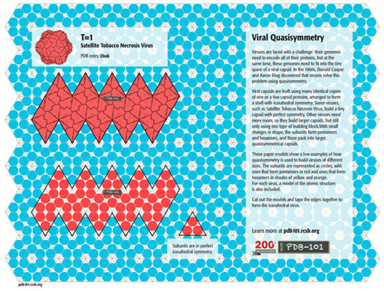
Protein subunits (capsomeres) of polyhedral viral capsids vary in their configuration, so we decided to focus on the 20 simple equilateral triangular pieces of an icosahedron. If you look at the detailed protein structure of capsomeres of a T1 virus such as the Satellite Tobacco Necrosis Virus (Figure 8), the inter-actions between capsomeres involve non-covalent boding through ionic interactions, positive-negative polar associations, hydrogen bonding, and van der Waals hydrophobic residue interactions. Thus, we used magnets between our capsomere models as with Olson’s group’s interactive meso-scale models of self-assembling polyhedral viral capsids [22,24,25,26] at the Scripps Research Institute in La Jolla, CA. They produced beautiful self-assembling dodecahedra. As delightful as these models have been for both the research and education they stimulated, we felt that icosahedral models would better represent the different members of the polyhedral viral capsid family. Thus, as original work in this area, we have modeled the self-assembly of a T1 Satellite Tobacco Necrosis Virus in three different ways.First, we [27] constructed a self-assembling icosahedron (Figure 9; Supplemental Movie S1). We use a Schlegel diagram (Figure 10) to construct a topological model of where to place the magnets so that all identical subunits align and bind. As was previously done with Olson’s dodecahedron model [22,24,25,26], by reversing the location of north and south poles of all of our magnets, we can construct two different enantiomers of the self-assembling icosahedron. See Tibbits [11] (pp. 80–82) for a similar experiment with two different enantiomers of the self-assembling dodecahedron.

After numerous unsuccessful attempts to produce self-assembling polyhedral, we have developed five design criteria:

First criterion: we must consider the need for a magnet map of complementary attracting and repulsing orientations. To determine which magnets should attract each other to form our complete structure, we used Schlegel diagrams because they preserve the topology of the configuration so that we can determine which subunits specifically bind to one another.

Second criterion: maintain a rotational symmetry of each subunit in the model.

Third criterion: design each subunit so that they are all identical to each other.

Fourth criterion: design each subunit so that it assembles into a sphere. We have found that having subunits with convex faces increases the odds that the magnets in two separate subunits will interact with each other when shaken in a container.

Fifth criterion: Self-assembly occurs in an environment. Therefore, the configuration of the vessel (both its shape and size) that the pieces are shaken in matters enormously in determining the time to produce full polyhedral. This is akin to a “ship-in-a-bottle” problem. (Table 3 and Figure 11).

Thus, self-assembly occurs not only much faster on average in spherical containers than in cylindrical containers, but the several of the experiments in cylindrical containers were not successful in generating complete icosahedra.

Combined, these five criteria help to increase the speed at which a given design correctly self-assembles, as the pieces can assemble in many different orientations. For each of the five Platonic solids one can glue a north facing and a south facing magnet on each edge of a convex subunit to achieve these goals. We have, for the first time, successfully produced self-assembling tetrahedra, cubes, octahedra, dodecahedra, and icosahedra models based upon these criteria.

However, to better model polyhedral viral capsids we wanted to build models using rhombic cells (icosahedral asymmetric units) such as shown in Figure 3 for a T1 virus. Therefore, we built a self-assembling decahedron of ten rhombi made by simply dividing a sphere into the 20 equilateral triangular faces but keeping ten pairs glued together (Figure 12a) and by developing asymmetric rhombi similar to those illustrated in many virology journals (Figure 12b).The decahedron model of subunits (Figure 12c) with knobs and holes was an important intermediate step in our research to develop a full sixty subunit T1 icosahedral model (Figure 13).

Self-assembly in each of these cases is a parallel process as the subunits are simply shaken together in a container with no one directing which subunit is interacting with any other one. To avoid human mediation, we often do the shaking in a rock tumbler or shaker bath to maintain randomness. When we do shake subunits by hand and intermediate dead-ends occur (such as four pentagonal assemblies of five triangular pieces), in order to assemble a full icosahedron, we break them and start over again. We also did this when using the rock tumbler because it becomes apparent after a certain amount of time tum-bling that some “bad” intermediates will not break apart on their own. We believe that these biomimetic models of self-assembling polyhedral not only help us better understand how viral capsids assemble in vivo, but illuminate how we might build nano-polyhedra for drug delivery that both assemble a priori and easily disassemble a posteriori at a target site with an external stimulus.

4.2. Parallel Self-Folding

We tackled the self-folding portion of this problem, thinking about self-folding nets of the platonic solids in an attempt to clarify and consolidate the existing literature, standardize existing notation, and provide new insights on what nets fold best.

By 3D printing a Dürer net of an icosahedron from polypropylene filament in two successive layers (the first layer is thinner and be-comes a series of hinges) (Figure 14) and dropping it into warm water, the net automatically folds into a 3D icosahedron. For such self-folding models we have had to set the direction of the first printed layer so that it is not parallel to any edge in the net. If the first (hinge) layer is printed with lines parallel to the direction of the living hinge, then the hinge will quickly break.

Prior to our work, many of the self-folding models in the literature required high tech spaces involving tiny models made from difficult to use materials such as solder or DNA. Our models can be printed in a middle school with a $50 roll of polypropylene filament and $10 of magnets. This work makes self-folding models much more accessible.

To consider self-folding, we need to understand that the number of Dürer nets explodes combinatorially (Table 2 above). Thus, the primary design challenge is to determine which Dürer net is able to fold faster to form a complete polyhedron with the least chance of forming intermediates that are unable to continue to self-fold. To distinguish each of the 43,380 Dürer nets of dodecahedra and the 43,380 Dürer nets of icosahedra, we use the Hamiltonian circuit of the degrees of the vertices (Figure 15).Unfortunately, there is a confusion in the literature in the definition of a vertex connection (Figure 16). Many articles define a vertex connection as a place on the net where two faces share a vertex but do not share an edge [29,30]. This works well for nets of the dodecahedron where there is only one way for such a joining of faces to occur, creating a 36° angle. This is also fine for nets of a cube, in which vertex connections only occur with the formation of 90° angles. Applying this same definition to nets with triangular faces results in two different types of vertex connections for the octahedron and three different types of vertex connections for the icosahedron. In the case of the octahedron, under the classical definition, vertex connections can be formed when three faces share a vertex forming a 180° angle, and when four faces share a vertex forming a 120° angle. For our purposes, we wish to only consider the more acute angle. Likewise, the first definition of vertex connections allows 180°, 120°, and 60° angles to be considered vertex connections for the icosahedron. Categorizing all three of these different types of connections as vertex connections sacrifices specificity of categorization that we do not wish to allow. Specifically, we desire a second, generalized definition for vertex connections that results in only one type of angle vertex connection and can be generalized not only to the platonic solids but to the Archimedean solids as well. So for the dodecahedron we consider only 36° degree angles, formed at vertices of degree 4 in the Durer net, and for the icosahedron 60° degree angles, formed at vertices of degree 6 in the net. From this point forward the term vertex connection of a net is used to refer to a vertex of a net that is incident in that net to every face it will be incident to in the assembled polyhedron. That is, at a vertex connection, the only operation needed to be performed to complete the polyhedron locally in a ϵ ball about that vertex is the gluing of two edges to each other. The number of vertex connections of a net is then the number of vertices of degree 3 for a cube net, degree 5 for a cube net, degree 4 for a dodecahedron net, and degree 6 for an icosahedron net.

We can also measure the number of leaves on the spanning tree of a net. This is also a variable that highly relates to the compactness of the net and how well the net folds. A leaf only shares one edge with other polygons in a Dürer net.

All eleven Dürer nets of cubes and octahedra have been extensively studied by Dodd, Damasceno, and Glotzer [29]. They focus on the number vertex connections on each net (Figure 17).

Spanning trees are a concept from graph theory that can be applied to our self-folding situation as a way to represent Dürer nets. A graph G = is a collection of vertices V and a collection of edges E indicating which vertices have an edge between them. A spanning tree T = of a graph G is a subgraph of G (That is V′ ⊆ V and E′ ⊆ E) such that V′ = V, every vertex has at least one incident edge, and T has no cycles. That is, we say T is a spanning tree if it contains all the vertices of the original graph, and every vertex still has at least one edge connected to it, but there are paths that can return to their starting vertex without repeating a vertex along the way.

There are two different types of spanning trees we want to consider. The first type of spanning tree is that of a cutting tree. A cutting tree represents the edges you would cut along to unfold a solid into a planar Dürer net. If we created any cycles in this tree, then we would completely detach a face or a collection of faces from the rest of the net, so certainly our cutting tree cannot contain any cycles. Additionally, the Dürer net must lie planar across its entirety. Therefore, since any closed solid is not locally planar at each vertex, at least one edge must be cut along so that the net will lie planar there. Therefore, every vertex of the polyhedron must be visited with no cycles. So the cutting tree is a spanning tree of the graph G = where V is the set of the polyhedron’s vertices and E is the set of the polyhedron’s edges.

Another way to visualize the relationship of a spanning tree on a 3D polyhedron to a 2D Dürer net is that instead of doing an edge cut, we can cut 3 of the 6 faces of a cube to form 6 triangular faces. The resulting Dürer net has a spanning tree of length 9 instead of 4 to 6 as shown in Figure 17 (Figure 18).The other type of spanning tree is a skeleton graph. In this case, we take the Dürer net itself and create a graph that represents it in the plane. We place one vertex at the center of each face on the Dürer net, and we connect two vertices with an edge if those two faces are connected in the planar Dürer net (Figure 1, Figure 2, Figure 14, Figure 15, Figure 16, Figure 17 and Figure 19). Since the net must lie planar and every face must be included for it fold to the completed polyhedron, the skeleton graph is a spanning tree.A spanning tree helps us generate two other useful topological invariants of Dürer nets. In graph theoretic terms, the diameter of a graph is the maximum taken over all pairs of vertices vi,vj of the minimum distance between vi and vj. However, since the skeleton graph is a spanning tree, there are no cycles and therefore it sufficient to define the diameter as just the length (measured in edges) of the longest path possible that does not repeat any vertices. We could consider this path the backbone of the skeleton (Figure 19).

For a given tree, it is possible for there to be multiple maximal paths. Thus, some skeleton graphs can have multiple backbones.

Another useful property of a spanning tree is its Degree Distribution. If we consider the spanning tree, in graph theoretic terms, then we can consider what the possible degrees of the vertices of the spanning tree of a Dürer net could be. A cube has 6 faces ⇒ Spanning tree has 5 edges If A is the number of vertices of degree 1 (leaves), B = number of vertices of degree 2, C = number of vertices of degree 3, etcetera, then we can therefore write two linear equations:This system of equations has only 4 discrete solutions that do not violate linear algebra and that can be represented as a valid net. In Table 4, we show the four satisfactory solutions and in Table 5 we give the number of possible degree distributions for each type of Platonic solid.Menon et al. [31], Pandey et al. [32], Kaplan et al. [33], and Pigrim et al. [34] used vertex connections and geometrically, the radius of gyration (Figure 20). Pandey et al. [32] define a net Ω’s radius of gyration by the following integral which computes a measure of how well packed the net is around its center of mass:

Rg2=∫Ωx−x¯2+y−y¯2dA

Other researchers [35] have slightly simplified this formula, by taking a summation over the centroids of the faces of the net instead of an integral over the whole net. We use this computation instead of the integral one because it produces nearly the same ranking of nets from least to most compact, while only sacrificing a small amount of specificity.

Rg2=1N∑i=1Nxi−x¯2+yi−y¯2

In this formula, N is the number of faces in the Dürer net, xi,yi is the center of the ith face of the Dürer net under some arbitrary enumeration of the faces, and x¯,y¯ is the center of mass of the entire net. This formula does the same computation of the first, but instead of integrating over the entire net, it just performs the calculation for the center of each face. Regardless of definition used in the literature, several independent studies have found a strong correlation between a decrease of Rg and an increase in the rate of successful foldings. In our data on the radius of gyration for various Dürer nets, we used the computationally simpler summation equation. One discrepancy in the literature is that both of these formulas are quadratically dependent on the side length of the faces of the net. Therefore, when researchers calculate the radius of gyration for a net, it is comparable to other nets in their paper, but may not be comparable to another researcher’s results who has used a different side length in their experiment. Therefore, we propose a normalization of the side lengths to 1 unit in this calculation. This allows radius of gyration of nets to be comparable between experiments even if the nets are printed physically with different side lengths. Regardless of definition, several independent studies have found a strong correlation between a decrease of Rg and an increase in the rate of successful foldings. Another way we can measure compactness geometrically is by considering the convex hull of a Dürer net. The convex hull of a Dürer net is the smallest convex polygon that encloses it (Figure 21).

We can measure both the area and the perimeter of the convex hull. Since the side lengths of a Dürer net are fixed to 1 unit in all of our calculations, then the area of the convex hull measures how much empty space is added that is not part of the Dürer net. This gives us a measure of how much space is “wasted” and thus a measure of compactness. However, the smallest area of a simple polygon is typically a thin rectangular shape, so while radius of gyration prefers more spherical compactness, the area of the convex hull picks up on more 1-dimensional compactness.

On the other hand, perimeter is minimized the closer the convex hull comes to being circular. Therefore, the perimeter of the convex hull has a very high correspondence with the radius of gyration. Graphs of linear regression of area and perimeter of convex hulls to radius of gyration.

Therefore, measuring radius of gyration, area of the convex hull, and the perimeter of the convex hull all tell us different things about how we might consider a particular Dürer net to be compact.

These geometric factors, however, are often driven by topological ones, which are the main factors we consider herein. These topological factors are the number of vertex connections and number of leaves on the net, as well as the degree distribution (Table 4) and diameter of the spanning tree of the net (Figure 16). Instead of using the radius of gyration as a geometric factor, we use the more visually easier to conceptualize: the area and perimeter of a convex hull of the net. Statistically, both the area and perimeter of a convex hull of the net are so positively correlated with their respective radius of gyration that we do not feel anything is lost (Figure 22 and Figure 23).This confirms our hypothesis that the radius of gyration and area of the convex hull measure two different types of geometric compactness [35], whereas the perimeter of the convex hull captures an extraordinarily similar type of compactness as the radius of gyration. Since the relationship between the perimeters of their respective convex hulls was much stronger than that of areas and captured much of the sense of the radii of gyration, we primarily use the perimeter of the convex hull as our geometric measure in our exploration of folded structures.

As defined above, we have identified seven topological and geometric variables that play a role in measuring a nets compactness and how well it folds.

While Menon et al. [31], Pandy et al. [32], Kaplan et al. [33], and Pigrim et al. [34] analyzed the folding of dodecahedra and icosahedra, they only examined models with the maximal number of vertex connections. Therefore, we chose to investigate the examples of self-folding of dodecahedra of all nine categories of Dürer nets from 2 to 10 vertex connections with different perimeters of their convex.In experiment, true parallel self-folding rarely occurs due to limitations induced by inertia, and thus more closely resembles inverted radial serial folding. In Figure 24, even if folding begins simultaneously across the surface of the net, the outer panels will begin to lift first. This is because for the net to fold along the red-blue edge, only one panel must be lifted. However, to fold along the red-green edge, 2 panels must lift, and to fold against the green-yellow edge the assembly pathway has to resist the inertia of three panels. Ultimately, to form the folded polyhedron, the outer panels need to travel farther than the inner panels.In addition to the 3D-printed Dürer net of an icosahedron that we described above (Figure 14) that successfully self-folds into a complete icosahedron, we have successfully printed two different Dürer nets of dodecahedra that partially and fully self-fold (Figure 25).