
 The spatial resolution, corresponding to the pixel size, was 30 m for Bands 1–7, 9 and 10, while it was 15 m for Band 8 (panchromatic) (
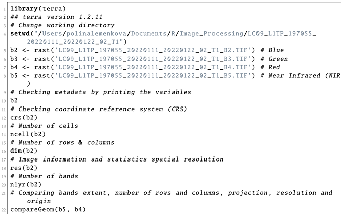
 Afterwards, the layers were read in the ‘landsat’ object class of R, where they were represented by the bands of the Landsat-9 OLI image. The reflection intensity had the following wavelengths: Ultra Blue or coastal aerosol (Band 1), blue (Band 2), green (Band 3), red (Band 4), near infrared (NIR) (Band 5), Shortwave Infrared (SWIR) 1 (Band 6), Shortwave Infrared (SWIR) 2 (Band 7), panchromatic (Band 8), cirrus (Band 9), Thermal Infrared (TIRS) 1 (Band 10) and Thermal Infrared (TIRS) 2 (Band 11). The visualisation of single bands was performed using Listing 3 and is presented as a subplot of grayscale scenes in
 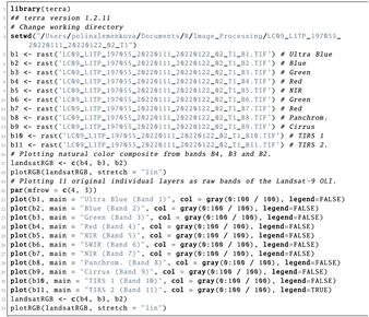 There was a difference in nuance between the grey corresponds and the numerical values and range of pixel values in diverse channels of Landsat. This is explained by the spectral reflectance that differs in various bands for objects on the Earth’s surface. Due to the individual reflectance of solar radiation by these features, the values differed accordingly. Such effects from spectral reflectance enabled us to use combinations of various bands to better represent the diverse phenomena and objects on Earth. For instance, the particular applications of Landsat bands are for geology (SWIR (Band 7), NIR (Band 5) and red (Band 4)) [
 Visual inspection of the satellite image product built from the monochrome image data (
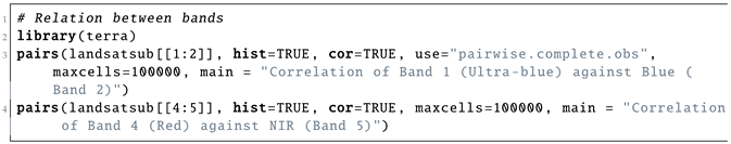
 3.3. Terrain Analysis in PythonTo model the relationship between the topographic variables and appearance, we applied Python algorithms for processing SRTM data by the 3D approach. Two different types of local features were computed for the SRTM image, namely the DTM and hillshade, with artificial light imitating the Sun’s illumination. The 3D visualisation of the terrain surface is changed by varied azimuth and altitude of sun. Technically, the terrain analysis has been performed using integration of several libraries of Python: EarthPy [
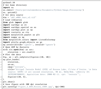

記住我


To cope with a series of Landsat bands and search for metadata, we examined the image parameters using regular expression with the command line utilities of Unix as a combination of grep, the Geospatial Data Abstraction Library (GDAL) and echo (Listing 1). Here, grep searches for text in a file according to a given pattern of characters, the GDAL filters spatial information in the dataset, and echo outputs the strings using the defined arguments.
Listing 1: Unix shell script by GDAL and echo-grep utilities to inspect the geometry of Landsat TIFs.The properties of the image were evaluated using a SpatRaster object by the R commands presented in Listing 2. Here, we inspected the CRS, the geometry of the image (number of cells, rows and columns) and extent, resolution and origin of the bands. The panchromatic channel (Band 8) had a higher resolution (15 m) compared with the set of the multispectral bands in the visible and thermal bands of the spectra (30 m). To ignore this difference in the matrix of the image, the raster in Band 8 (panchromatic) was resampled to the structure of the same number of rows and columns as in other bands (Here, target Band 1 is in Ultra Blue) by creating the RasterBrick multi-layer object as demonstarted in Listing 2.
Listing 2: R code used for inspecting the information and statistics on the Landsat 8-9 OLI bands.Subsetting large files, such as multispectral Landsat images, was performed using the SpatRaster object and ’subset’ function, which enabled processing the necessary bands of the Landsat image. In this respect, it enabled ignoring the cirrus, TIRS and other bands that were not relevant for a given task and to leave only the visible spectra. In this way, a subset of the target layers was selected from the SpatRaster object, while other bands were removed from the dataset using Listing 4.
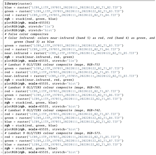
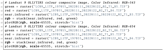
Listing 4: R code for subsetting the large files using SpatRaster object.Since there was not much information in the monochrome bands of the Landsat OLI/TIRS image, they were combined into colour composites to create more representative images. Plotting of the colour composites was based on the combinations of the three bands used as elements of the matrix scene. The three bands assigned to each of the three primary colours (red, green and blue (RGB)) were displayed with images using Listing 6.
Listing 6: R code used for plotting the color composites for bands of the satellite image.The vegetation indices were computed based on the arithmetically transformed combination of Landsat OLI/TIRS bands. This resulted from the existing formulae for band computations using mathematical operations with bands. The map algebra included addition, subtraction and division of the brightness in cells of the NIR and red bands of the Landsat image. The differences in the bands highlight the regions of the enhanced and more healthy vegetation in the target area of the image, which presents information for environmental monitoring. The resultant image shows brightness values of vegetation modified by colour palettes made using arithmetic operations on the composite bands.
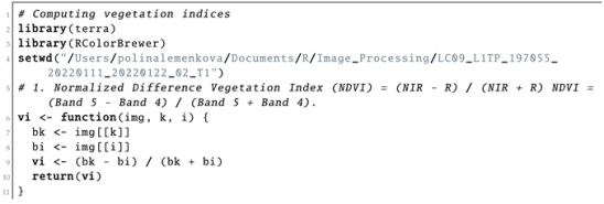
The most widely used and well-known vegetation index is the Normalised Difference Vegetation Index (NDVI), which applies the ratio of the difference in values between the red and NIR bands and their sum. Similar to the NDVI, the Enhanced Vegetation Index (EVI) quantifies vegetation greenness with added corrections for the atmospheric conditions and canopy background noise. Aside from that, the EVI is more sensitive in forest areas with more dense canopies and vegetation coverage, which is useful for the forest regions of Côte d’Ivoire. The Soil-Adjusted Vegetation Index (SAVI) is built up by using the NDVI and correcting for the effects of soil brightness in the regions where vegetative cover is low, namely deforested areas and the fragmented savannahs of Côte d’Ivoire. The Atmospherically Resistant Vegetation Index 2 (ARVI2) is the most applicable index in regions with high atmospheric aerosol contents. Examples of other environmental indices include the Normalized Difference Water Index (NDWI), modified Normalized Difference Water Index (MNDWI) and Water Ratio Index (WRI) [125].Computing the vegetation indices is an important environmental tool which is based on information from the DN values of pixels, indicating the spectral reflectance of the red and NIR bands as measured by the sensor. It is commonly computed with the spatial statistics and algebra of the bands using the cell values of the image as shown in Listing 7. The reason for selecting the NIR and red bands for computing the vegetation indices is vegetation appearing brighter in these bands, since it reflects more energy in the NIR and red bands compared with other wavelengths. Contrarily, water absorbs most of the energy in the NIR band and is therefore represented by black to very dark brown colours. Through a series of interactions among the elements of an image, they are allocated to the classes based on the weighted values of their relative proportions.
Listing 7: R code used for computing vegetation indices from bands of the satellite image.The geospatial TIFF was visualised for modelling the DEM as GeoTIFF using the Rasterio library, which imported the dataset as a raster array of cells, read the GeoTIFF format and stored a gridded raster as a digital terrain model (DTM) or satellite images (Listing 8). The elevation data were imported by Rasterio as height values that were contained in the cells of the corresponding raster. The structure of the data presented a NumPy array in the form of a matrix with the DNs of pixels. The terrain was plotted as an array of cells representing the land surface according to the elevation values, as shown in Listing 8. Plotting of the bands was performed using the ep.plot_bands() function using the spatial dimensions of the raster file.
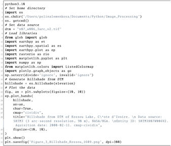
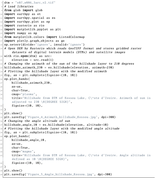
Listing 8: Python code (1) used for plotting DEM in Figure 2.The hillshade was calculated using the altitude of the Sun as a light source at the zenith and azimuth of the illumination source (Listing 9). The functions to compute the variations between the exemplar locations of artificial illumination of the terrain resulted in the visualised details of the terrain in the Kossou Lake surroundings. The slope and aspect of the terrain were used as auxiliary variables for the terrain modelling. The hillshade modelling was inherently related to static cartographic representations of the Earth’s topography, and thus hillshade was used for the geomorphometric representation of the terrain of Côte d’Ivoire.
Listing 9: Python code (2) used for plotting hillshade in Figure 3.Hillshade represents the terrain with a hypothetical illumination value in the monochrome scale (0–255) with cells on the raster scene showing the terrain surface with a given specified light source. The illumination was changed to 10° and 230°(in radians) to better represent a geospatial model of the topographic relief of Côte d’Ivoire (Listing 10). Assume that the orientation differences between the angle and azimuth of artificial illumination in modelling the topography of Kossou Lake are independent and identically distributed according to the time and seasonal parameters. To visualise the characteristics of the relief in the topographic model based on the DEM, raster data were sampled to estimate the variations in distribution of the parameters. In our case, we selected azimuths of 10° and 230°. We observed that the effects from the contrasting variations in relief approximately followed the changes in the Sun’s azimuth and angle altitude.
Listing 10: Python code used for plotting the hillshade with changed azimuth and Sun angle values for Figure 4 and Figure 5.We assumed the data to be of a high resolution, which may have presented our current limitations. However, the precision may affect the resulting topographic model through coarser resolution data (i.e., lesser meters in one pixel will give a rough representation of the Earth’s surface and miss smaller landforms in the landscape). Regarding this, it is strongly recommended to apply very high-resolution data for a precise representation of the Earth. Another point of concern consists of selecting the correct view shed and azimuth for modelling the aspect, slope and elevation, which is especially true for mountainous regions and rugged reliefs. Although the Python-based method of terrain modelling can potentially handle materials with coarser or unknown resolutions for the original data, the results may hide the selected structures on the Earth’s surface. The same issue concerns the applications of R for image processing, where the precision of the output data corresponds to to the original resolution of the input data. In our future works, we are very interested in extending our study to handle higher-resolution imagery, such as Sentinel 2A at a 10 m resolution or Satellite pour l’Observation de la Terre (SPOT) with up to a 1.5 m spatial resolution in the panchromatic and multispectral channels.
In the presented methodology, we applied Python and R algorithms which process and model the terrain characteristics of the Earth using the spatial parameters of the remote sensing data. By exploiting the spectral reflectance characteristics of the satellite bands, we used information from the Landsat channels from the corresponding cells which represent objects located on the Earth. Interpretation of these values is based on their spectral reflectance in various wavebands, which provides information on the characteristics of typical land cover types. This was possible through the analysis of the different brightness of each land cover type (e.g., forests, rivers, lakes and other water bodies or urban spaces). In turn, the geomorphometric models formed using Python scripts enabled predicting the distribution of various soil properties and associated vegetation types which were related to the specific slope steepness and regional topographic features. Examples of the application of terrain models include hazard risk assessment in applied geology for erosion, landslides and avalanches in mountainous regions. The major advantage of using Python and R scripts for environmental modelling is that it reduces the time of data processing and increases the precision of models through automation of data processing, because scripts are repeatable for other regions and can be applied in similar studies.
5. ConclusionsIn this paper, we proposed two scripting approaches to satellite image processing to compute several vegetation indices and to perform terrain modelling. The scripting techniques of the ’raster’ and ’terra’ packages of R for computing vegetation indices demonstrated great potential for using map algebra and calculation techniques with the Landsat OLI/TIRS for monitoring vegetation health and environmental mapping. Moreover, this technique is also useful for agricultural applications where deteriorated sites may require remediation or close monitoring. To model terrain variables, we proposed a Python-based approach where the topographic data are derived from the SRTM DEM using the EarthPy library.
The problem of the terrain analysis in image processing can be referred to as spatial data modelling, with classification of cells according to the elevation values. The derived variables are essential for visualisation of the slope, aspect and hillshade using the parameters of the Sun’s angle and azimuth. Mapping the topographic data using terrain analysis by Python highlighted their fundamental importance in Earth modelling. Thus, the relief of the Earth’s surface has notable effects on various components of the ecosystems, including geological, climatic and hydrologic processes as well as the soil vegetation parameters. Moreover, topography regulates and controls climate processes such as precipitation, wind direction and strength. Therefore, it plays a crucial role in the environmental dynamics and ecosystem functioning, which includes the uneven distribution of the diverse landscapes with contrasting types of vegetation in the hilly and coastal areas of Côte d’Ivoire.
The integrated use of regional environmental resources presents the potential for sustainable development of Côte-d’Ivoire. This requires regular monitoring of the environmental conditions of the country using satellite images. In data science, processing satellite images using advanced programming methods is a challenge which consists of adaptation and optimisation of the programming algorithms towards spatial data modelling and analysis. In this study, we presented a solution to this problem with a straightforward yet effective approach which combines libraries of Python and R for processing RS data in a scripting framework. The use of both programming languages allowed us to use the best packages for topographic and environmental modelling separately when handling the satellite images. It also demonstrated the integration of the spatial libraries of the two scripting languages for terrain mapping and image processing aimed at environmental data analysis.
The techniques of R enabled image processing using information derived from pixels in the image scene. Spatial data were differentiated by the RGB triplet colours through plotting the colour composite of the Landsat 8 OLI/TIRS image using the R library ’raster’, which adapts the general syntax of R for spatial data processing. The colours corresponded to the composites of the RGB signals scattered from the natural and built-up environment, which resulted in various DN values for the pixel cells in a raster matrix of the image. The combinations of the three channels were tested by the R library ’terra’ as sensor bands, which displayed the image and visualised the appearance of various terrain objects using the distinct colours. We compared the correlation between the selected bands of Landsat-8 OLI/TIRS C1 in a multispectral image for Bands 1 and 2 (blue and green) and 4 and 5 (red and NIR). We then computed four selected vegetation indices—NDVI, SAVI, EVI2 and ARVI2—using the principles of map algebra based on the DNs of the reflectance values of the pixels in the selected spectral bands (NIR and red). The major effect of spectral reflectance from healthy green vegetation was visible in the NIR region of the image spectrum, with a strong NIR response rising sharply for healthy vegetation. Conversely, the areas with poor or damaged vegetation were represented by a low NIR response, which notably decreased as shown by the vegetation indices and with corresponding lower values for the NDVI.
The algorithms of the EarthPy library of Python were used for terrain modelling based on the high-resolution SRTM DEM. The upscaled mapping was shown at the two hierarchical levels: regional environmental analysis of the Yamoussoukro surroundings and local topographic modelling of the Kossou Lake. Processing the topographic data for visualisation of the slope, aspect, hillshade and elevation was based on interpolation of the cell values in a raster matrix grid to spatial polygons that corresponded to the diverse terrain structures. We showed these methods in a series of scripts with detailed explanations of their functionality and the effects of changed parameters on the image. The main advantage of Python for spatial modelling consists of the machine-based automation of data processing. Specifically, it derives information from the satellite images in an efficient way using a straightforward syntax, which enables handling complex RS data. The nonlinear environmental and topographic links among the near-surface processes could be depicted from raster matrices of the satellite images using programming algorithms. This enabled us to highlight the complex relationships between the objects forming the terrain shape and the diverse landscapes on Earth.
A wide variety of Earth’s features can be mapped using satellite images: climate change, urban sprawl, degradation of vegetation, deforestation, topographic variations or land cover change. At the same time, the analysis of the complexity of a particular phenomenon requires advanced methods of data processing to reveal the links and correlations among the objects and to map spatial patterns. For instance, topographic variations may be caused by geologic effects and anthropogenic activities, or the environmental dynamics of the Earth’s landscapes may involve nonlinear long-term and short-term variations. The comprehensive analysis of such processes requires advanced automatic processing of large datasets, where a conventional GIS is not effective enough. At the same time, due to the high level of spatial detail, high-resolution satellite images require efficient algorithms for data handling, including image resampling, band composition, statistical processing and map algebra for calculation of the vegetation indices. This requires the advanced methods for image processing made possible by programming languages.
As we demonstrated, the effective way to handle this issue includes the use of high-level programming languages such as Python and R. Scripting libraries are effective for automatic image processing and retrieval of spatial information from satellite images. The advanced algorithms of Python and R can be successfully used for processing Earth observation data and geospatial modelling in a robust, automatic and effective way. The application of programming approaches for terrain analysis and environmental monitoring is successful in dealing with multispectral RS data. The advantages of Python and R in image processing include scripting algorithms which ensure automation of RS data processing. Compared with GISs, the functionality of Python and R were proven to have robust handling of the geospatial data due to the high speed and effectiveness of code and repeatability of the scripts, which outperformed the existing state-of-the-art approaches of the traditional software.
In future works, we plan to use combinations of other libraries of Python and R for higher-resolution images, such as Sentinel-2A or SAR data for environmental mapping of the tropical forest regions of Africa. Specifically, we intend to focus on the long-term analysis of the environmental dynamics using time series of satellite images. Spatial modelling of the large series of RS data involves challenging problems with regard of their processing. For example, it is computationally challenging to deal with big data and requires complex methods of data handling. To this end, we plan to develop effective approaches to process large spatiotemporal datasets using scripting languages. Our next work will continue the development of the advanced cartographic methods for processing satellite images with programming languages.
留言 (0)