
記住我


Conceptualization, Y.-C.K.; methodology, N.H.; software, N.H.; validation, N.H. and Y.-C.K.; formal analysis, Y.-C.K.; investigation, N.H.; resources, N.H.; data curation, N.H.; writing—original draft preparation, N.H. and Y.-C.K.; writing—review and editing, Y.-C.K.; visualization, Y.-C.K.; supervision, Y.-C.K.; project administration, Y.-C.K.; funding acquisition, Y.-C.K. All authors have read and agreed to the published version of the manuscript.
Figure 1. An overview of the proposed method. The input consists of a series of cardiac short axis slice images, which range from the out-of-apical slice level to the out-of-basal slice level. The slice levels were labeled as ‘oap’ for the out-of-apical slice, ‘ap’ for the apical slice, ‘mid’ for the mid-level slice, ‘bs’ for the basal slice, and ‘obs’ for the out-of-basal slice. For each slice image, a pre-trained deep CNN model is used as a feature extractor. The features are denoted by xi for i = 1, 2, …, N, where N is the number of slices. The RNN model takes a series of features (i.e., x1, x2, …, xN) as input and produces probability scores for each slice level via softmax. The red numbers indicate the maximum values in the output prediction scores.
Figure 1. An overview of the proposed method. The input consists of a series of cardiac short axis slice images, which range from the out-of-apical slice level to the out-of-basal slice level. The slice levels were labeled as ‘oap’ for the out-of-apical slice, ‘ap’ for the apical slice, ‘mid’ for the mid-level slice, ‘bs’ for the basal slice, and ‘obs’ for the out-of-basal slice. For each slice image, a pre-trained deep CNN model is used as a feature extractor. The features are denoted by xi for i = 1, 2, …, N, where N is the number of slices. The RNN model takes a series of features (i.e., x1, x2, …, xN) as input and produces probability scores for each slice level via softmax. The red numbers indicate the maximum values in the output prediction scores.
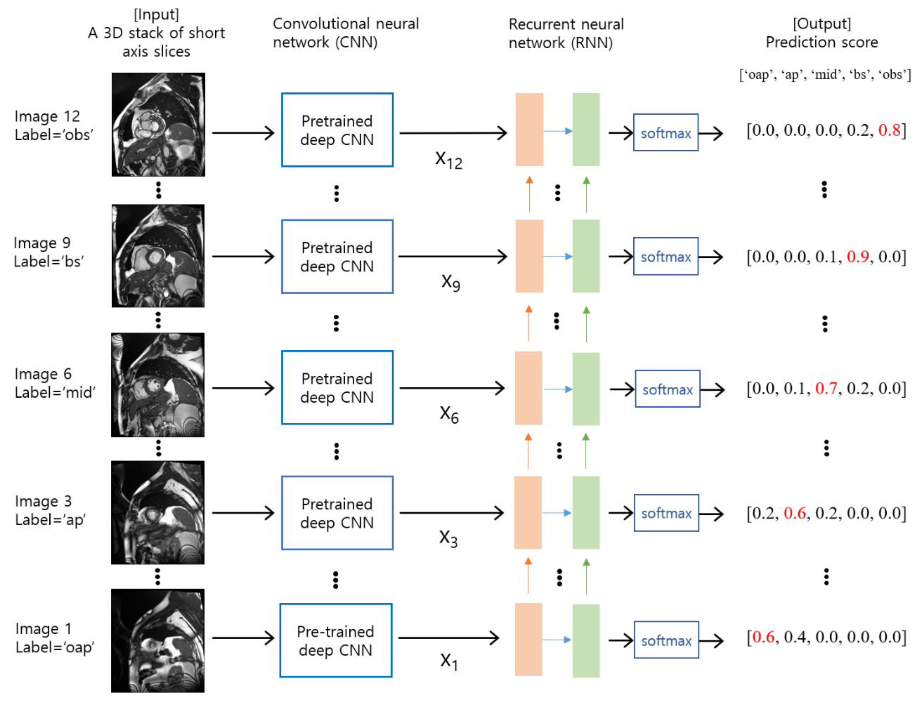
Figure 2. Learning curves for loss (top) and accuracy (bottom) when EfficientNetB0 was used as a baseline CNN architecture. Solid lines represent validation results, while dashed lines represent training results. Loss curves for EfficientNetB0 were not plotted because their loss value ranges were well above those for EfficientNetB0_2-LSTM and EfficientNetB0_2-GRU.
Figure 2. Learning curves for loss (top) and accuracy (bottom) when EfficientNetB0 was used as a baseline CNN architecture. Solid lines represent validation results, while dashed lines represent training results. Loss curves for EfficientNetB0 were not plotted because their loss value ranges were well above those for EfficientNetB0_2-LSTM and EfficientNetB0_2-GRU.
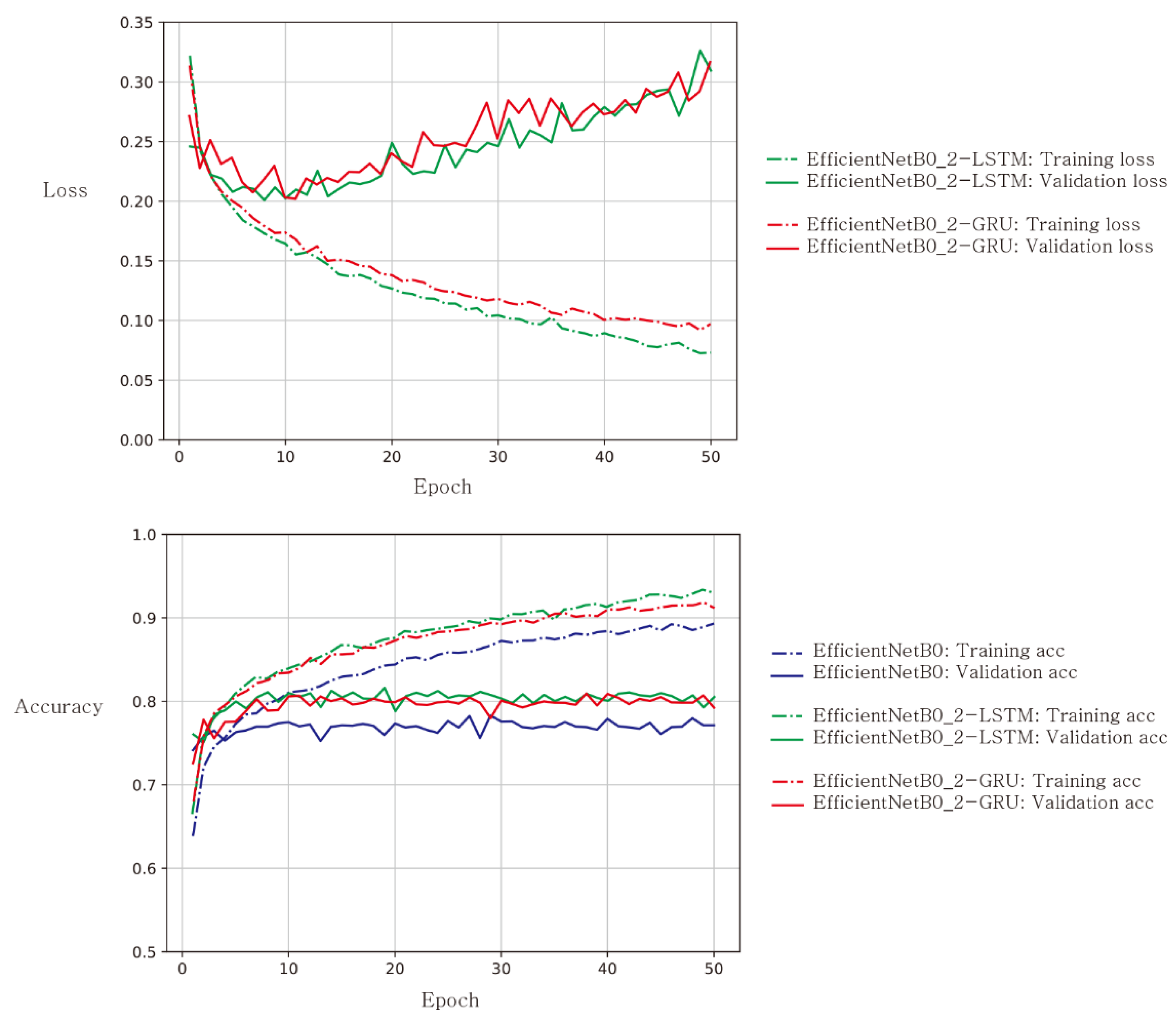
Figure 3. A screenshot of slice level predictions on a series of short axis slices on an individual test subject. The prediction was made by the ‘MobileNet_2layerLSTM’ model. The slice index, the ground truth, and the predicted category are shown above each image. The green text indicates correct classification, while the red text indicates incorrect classification. For example, ‘(BS) (P = OBS)’ indicates that the ground truth is ‘basal’, and the model’s prediction is ‘out-of-basal’.
Figure 3. A screenshot of slice level predictions on a series of short axis slices on an individual test subject. The prediction was made by the ‘MobileNet_2layerLSTM’ model. The slice index, the ground truth, and the predicted category are shown above each image. The green text indicates correct classification, while the red text indicates incorrect classification. For example, ‘(BS) (P = OBS)’ indicates that the ground truth is ‘basal’, and the model’s prediction is ‘out-of-basal’.
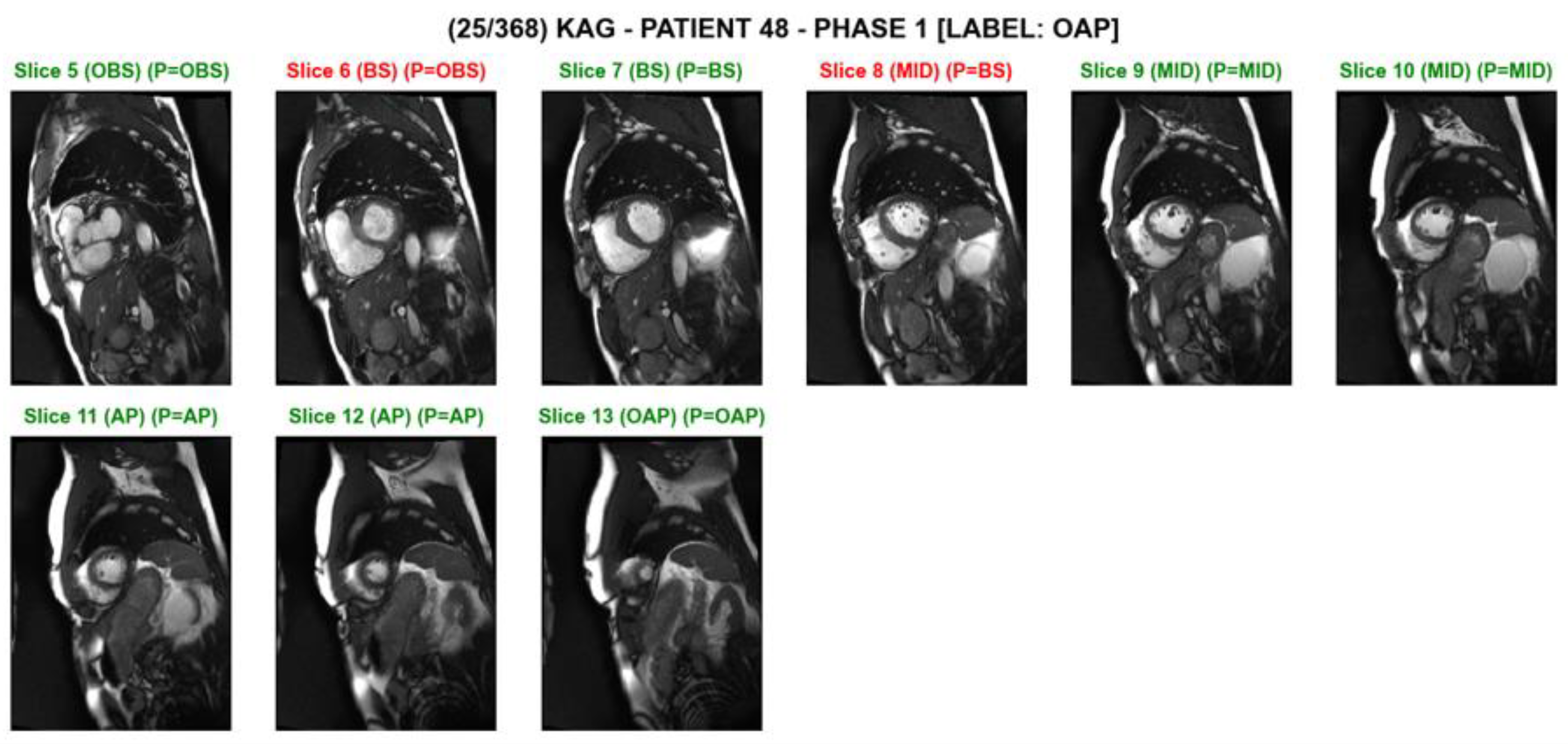
Figure 4. Test prediction results from the CNN-alone models (a,b) and from the CNN-RNN models (c,d). In either MobileNet or NASNetMobile, the CNN-RNN model has smaller sums of the elements out of the tridiagonal entries (SOTD) than the CNN-alone model. The elements out of the tridiagonal entries are indicated by the red contours in the confusion matrices. For example, SOTD is 11 for the case of MobileNet_2-LSTM in (c).
Figure 4. Test prediction results from the CNN-alone models (a,b) and from the CNN-RNN models (c,d). In either MobileNet or NASNetMobile, the CNN-RNN model has smaller sums of the elements out of the tridiagonal entries (SOTD) than the CNN-alone model. The elements out of the tridiagonal entries are indicated by the red contours in the confusion matrices. For example, SOTD is 11 for the case of MobileNet_2-LSTM in (c).
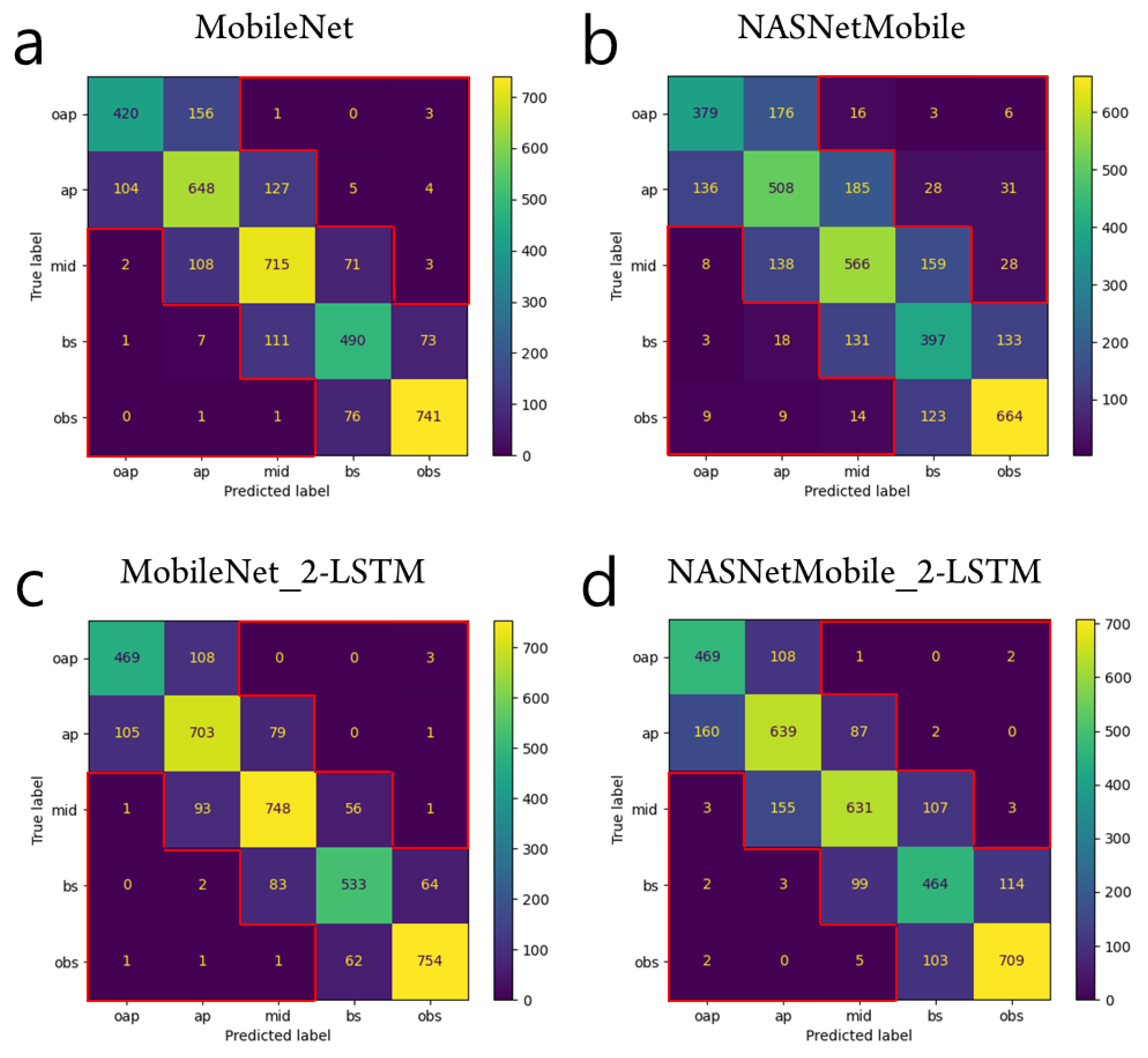
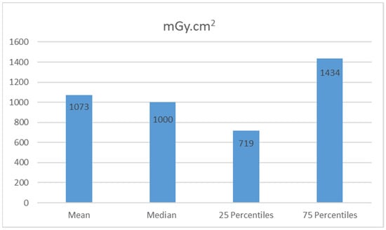
Figure 5. Comparison of SOTD values across deep learning models. SOTD was calculated to be the sum of the elements that are outside the tridiagonal entries. SOTD values were grouped by the type of the baseline deep CNN. The lower the SOTD value, the higher the prediction performance in general.
Figure 5. Comparison of SOTD values across deep learning models. SOTD was calculated to be the sum of the elements that are outside the tridiagonal entries. SOTD values were grouped by the type of the baseline deep CNN. The lower the SOTD value, the higher the prediction performance in general.
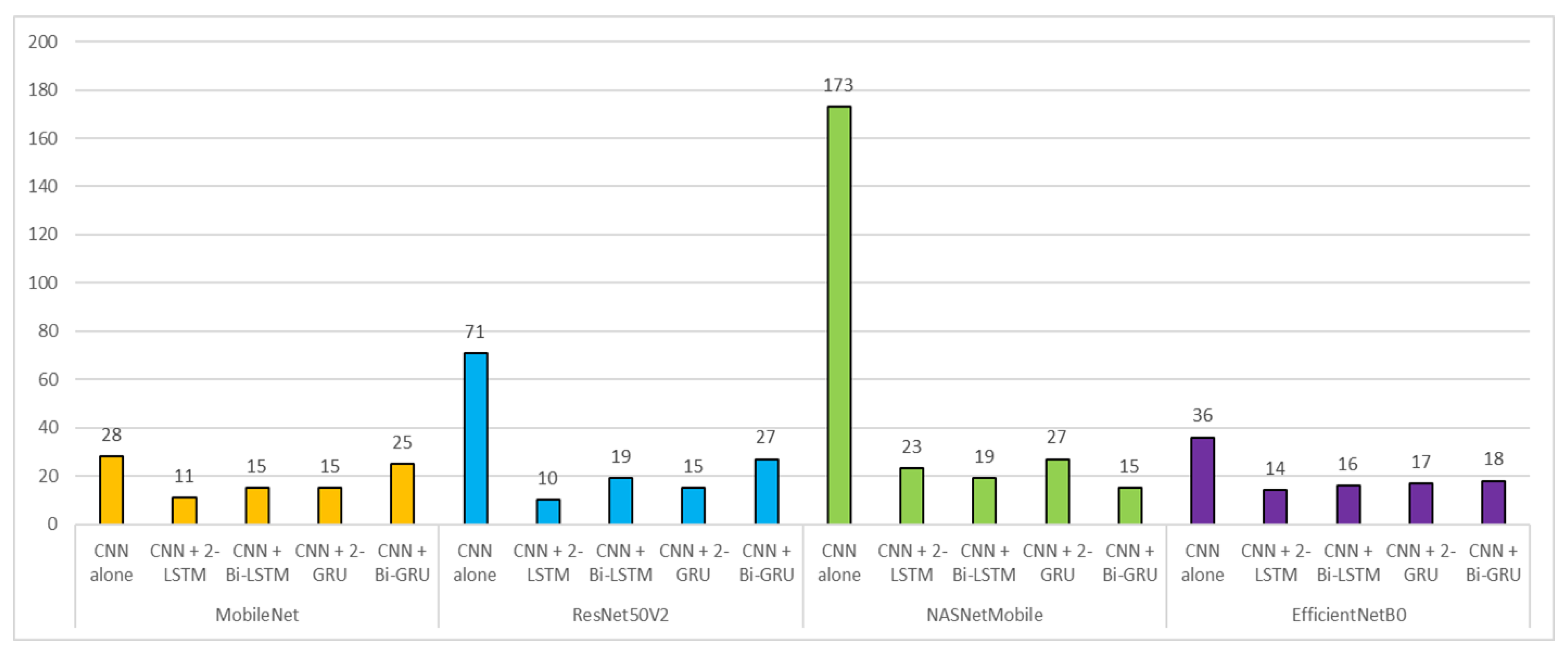
Table 1. The numbers of subjects in training, validation, and testing groups.
Table 1. The numbers of subjects in training, validation, and testing groups.
TrainingValidationTestingTotalNumber of subjects576214184974Percentage (%)59.122.018.9100Table 2. The numbers of samples in training, validation, and testing groups.
Table 2. The numbers of samples in training, validation, and testing groups.
Model Type TrainingValidationTestingTotalCNN *Number of samples12,0704594386820,532Percentage (%)58.822.418.8100CNN-RNN **Number of samples11524283681948Percentage (%)59.122.018.9100Table 3. The number of images for each class label in training and validation datasets.
Table 3. The number of images for each class label in training and validation datasets.
Class LabelTotal oapapmidbsobsTrainingNumber of images1878278428002132247612,070Percentage (%)15.523.123.217.720.5100ValidationNumber of images710108611147519334594Percentage (%)15.523.624.216.420.3100Table 4. The comparison of base deep CNN models.
Table 4. The comparison of base deep CNN models.
CNN Base NetworkNumber of Model ParametersImageNet Top-1 AccuracyNumber of Features after GAP *Batch Size for CNNBatch Size for CNN-RNNEfficientNetB05.3 M77.1%1280322MobileNet4.2 M70.6%1024322NASNetMobile5.3 M74.4%1056322ResNet50V225.6 M76.0%2048162Table 5. Prediction performance of a variety of deep learning models. The bold indicates the highest value among the models.
Table 5. Prediction performance of a variety of deep learning models. The bold indicates the highest value among the models.
CNN Base
留言 (0)