Incorporation of spatial- and connectivity-based cortical brain region information in regularized regression: Application to Human Connectome Project data

(depending on the hemisphere) and m = 2

• Signal strength σb2∈

• Variance of error σε2∈ (having a situation with stronger and weaker signals from the data)

• Parameter of dissimilarity diss(ACobs, ACtrue) = 0.25

• Fraction of the information coming from the connectivity rC ∈ , where part of the information coming from the spatial proximity is rD = 1−rC

We generate synthetic data according the specification below:

1. Matrix Z ∈ ℝn × p with iid rows from N(0, Ip)

2. Matrix X ∈ ℝn × m with iid rows from N(0, Im)

3. Coefficients vector b~N(0,σb2Btrue-1)

4. Coefficients vector β = (0, 0)T

5. Response vector y = Xβ+Zb+ε with ε~N(0,σε2In)

The settings above are considered separately for each of the two hemispheres. For a particular hemisphere, we find corresponding Laplacians based either on the structural connectivity or the distance. As in Karas et al. (2019), to evaluate the estimation accuracy, we study the relative mean squared error, which is expressed as

rMSE(b^)=||b^-b||22||b||22. (11) 3.2. Study of the estimation error and its components: Bias and variance

Mean Squared Error is the sum of the variance and squared bias. In addition to studying classical MSE measure of all the methods' estimates, we also examined its components to have a more comprehensive picture of the disPEER estimation quality, e.g., to see the relationship between the variance and squared bias.

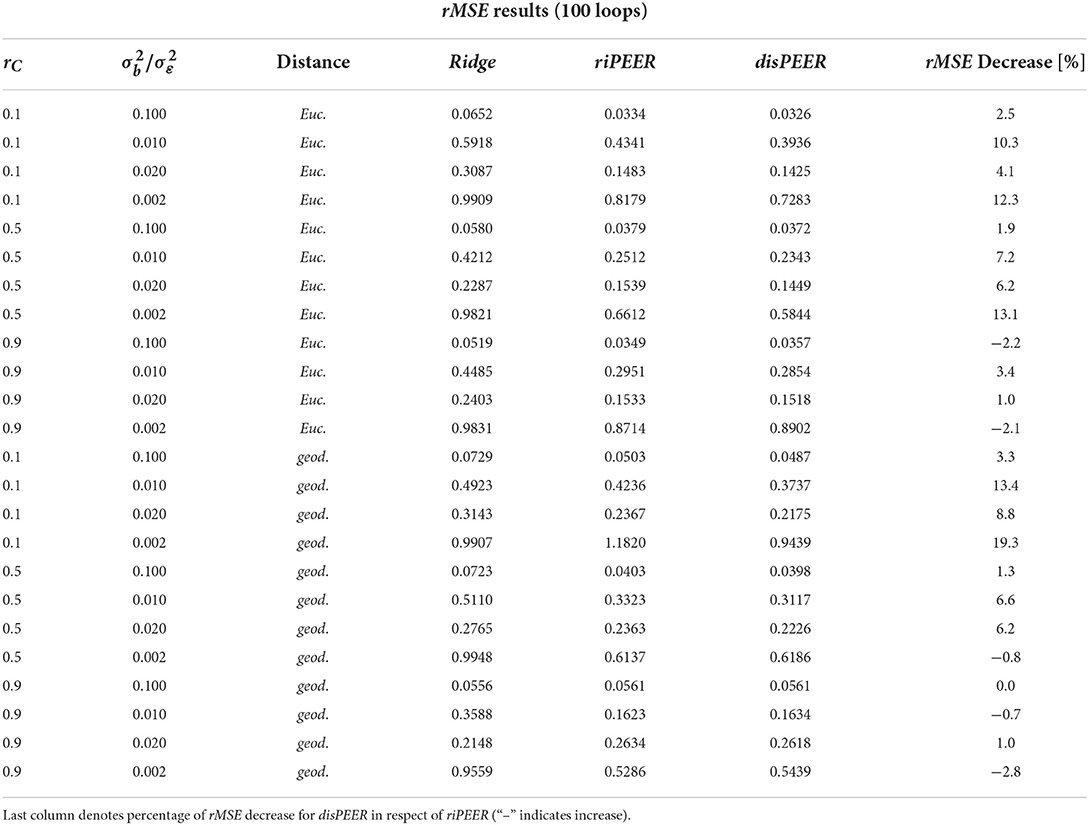
As Figure 6 shows, median rMSE of the b coefficient values estimates is lower for disPEER than either for riPEER or for ridge regression. It can also be seen from the results presented in Table 2 that for the majority of the settings disPEER shows the best performance. All these results are obtained under the assumption that we know the true value of the parameter h with which the proximity is determined. However, using different values of h in the estimation, we can still show better performance of our method (see Supplementary material). The results in Table 2 also show that the disPEER method works very well, especially for rC = 0.1, independently of the distance approach used. It is an expected behavior, as it is the setting where our method is supposed to work the best, because the relationship among the coefficients b is mainly driven by the information coming from the distance matrix. We notice that the rMSE percentage decrease reaches up to 20% compared with the riPEER approach. Even if we equally distribute origination of information for the generation of the b coefficients between both connectivity- and distance-based information, disPEER still prevails over its sister method riPEER. We also conducted experiments to study the behavior of rMSE when n ∈ (Supplementary Tables 1, 2). In these settings, the information content is smaller relative to the sample size and there are cases when ridge regression provides smaller rMSE than brain-information-based methods. This behavior is especially visible in the situations when the ratio of σb2/σε2 is the lowest, hence, the signal to noise ratio is small: σb2/σε2=0.002. Moreover, the number of cases when rMSE for riPEER and disPEER that are close to each other increased in comparison to n = 400.

FIGURE 6

Figure 6. Plots of rMSE (medians) of b estimates for different connectivity information configurations rC ∈ with σb ∈ , σε = 1, and h = 5 for ridge, riPEER, and disPEER (left hemisphere and Euclidean distance).

TABLE 2

Table 2. rMSE (median) results for ridge, riPEER, and disPEER methods with h = 5 and h = 100 for Euclidean and geodesic distances, respectively, for σb2∈ and σε2∈.

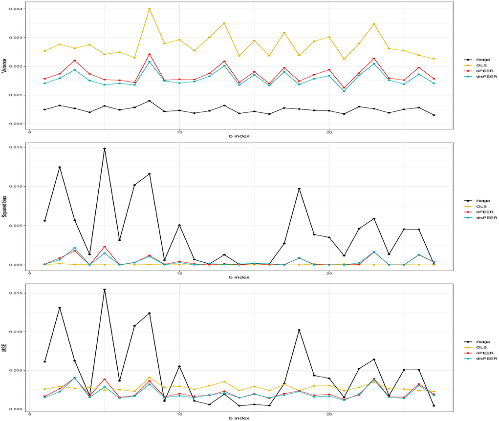
Figure 7 shows that our approach helps in keeping the balance between the variance and squared bias trade-off in contrast to ridge regression, which despite showing very low variance cannot cope with prominently higher bias (hence, worse MSE). Also, the distance-based approach has slightly lower variance than riPEER. We do not claim any theory-based properties here. However, our extensive simulation studies show that our new method, disPEER, shows improved performance when compared with other regularization methods. We cannot claim uniform improvement in every single case, but it is undoubtedly a prevalent phenomenon.

FIGURE 7

Figure 7. Empirical variance, squared bias, and MSE of b estimates for σb = 0.01, σε = 1, rC = 0.5, and h = 5 (left hemisphere and Euclidean distance).

Proximity parametrization—sensitivity analysis. In Table 2, we present the results for the true values of the proximity parameters h equal to 5 and 100 for Euclidean and geodesic distances, respectively. We chose these values, because we want to keep the distance information we give for coefficient estimation as useful as possible. In Figures 2, 4, one can observe that h should not be too large in the Euclidean approach, because more and more regions become close to each other and we lose the differentiation in the proximity matrix. In contrast, what happens with geodesic distance (Figures 3, 5) is that with the increase of h, we observe that proximities get decidedly more binarized. Our Supplementary Figure 2 shows that our estimation procedure is robust to the mis-specification of the parameter h.

3.3. Human Connectome Project data application

We want to compare the estimation methods presented in Section 2, especially the new method disPEER in the context of real data. Our aim here is to consider the numerical response, which is a particular measure of cognition. All analyses are adjusted for the demographic data (gender and age) with their coefficients unpenalized (fixed effects). Regression coefficients associated with the cortical volume are penalized (random effects). To perform this analysis, we will use the data from the Human Connectome Project repository (HCP). Also, we will use the data on the brain anatomic measurements: structural connectivity and brain cortical regions' spatial proximities. These data are not available in the HCP repository. To obtain these measurements, we used the pipeline developed and implemented by Dr. Goñi (Ramírez-Toraño et al., 2021).

3.3.1. Data description and preparation

As a part of the application of the studied methods on the imaging data, we used the publicly available data from the Human Connectome Project. This is a project funded by the National Institutes of Health HCP with the original goal of building a map of the neural connections and producing the data in order to study brain disorders. The HCP repository contains data on 1,200 young adults in the age range of 22–35. The data we use do not contain all the 1,200 subjects from the HCP study. Initially, we chose adults in such a way that we do not have related persons among them, so we analyzed only independent observations. It led to data from 428 unrelated individuals. Cortical properties and the cortical regions' coordinates in the HCP study were obtained using the FreeSurfer software.

We focus on both the cortical thickness and cortical area data as in further work we consider the volume which is the product of the thickness and the area. We found a few outliers in both hemispheres and we decided to replace their data with their family members' data or, in cases where this was not possible, we deleted such data from our analysis. As a result, we used 424 and 426 subjects in the analysis of the left and right hemispheres, respectively.

3.3.2. HCP data analysis

To achieve a meaningful interpretation of the disPEER's performance in the case of real data, we wanted to compare it with other statistical methods. We studied the estimation using Ridge Regression, Ordinary Least Squares assuming a linear regression model with coefficients [β, b], the riPEER method with fixed and random effects and a penalty term containing the Laplacian originating from the structural connectivity, and our proposed disPEER approach, also with a linear mixed model formulation and penalty component incorporating the structural connectivity and spatial proximity information. In the HCP data setting, the coefficients of Gender (categorical 0/1 variable) and Age (numerical variable), corresponding to X matrix, are not penalized. We penalize the coefficients of individual-brain-normalized cortical volume measurements (Z matrix), which are obtained by multiplying the average cortical thickness and cortical areas. We normalize regions' volumes by dividing every measurement by the subject's cortical volume in the particular hemisphere. This is because brain volumes especially differ between men and women; on average, men's brain have higher volumes than women's. As a response y, we chose the measurements of Language/Vocabulary Comprehension, which measures a participant's receptive vocabulary. The respondent is presented with an audio recording of a word and four images on the computer screen and is asked to select the picture that most closely matches the meaning of the word. In the estimation process, we used standardized variables (mean 0 and variance 1) in the X and Z matrices and outcome vector y. For riPEER we applied R package mdpeer with connectivity-based penalty-Laplacian Q~C. With the usage of this matrix and additionally a proximity Laplacian Q~D, we estimated model coefficients with disPEER.

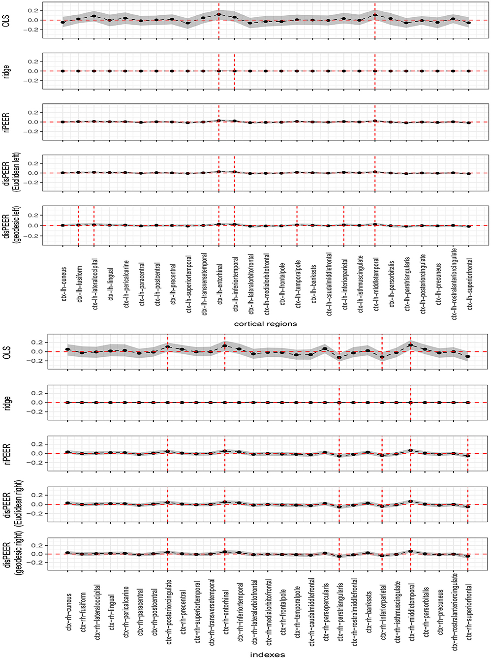
3.3.3. Estimation of the coefficients for language/vocabulary comprehension

Coefficient estimates obtained using disPEER for the left hemisphere turned out to be primarily driven by the proximity as was seen in the penalty parameter estimates. Coefficients indicated as significant in the right hemisphere are the same for both disPEER and riPEER Figure 8 which can be easily explained by the fact that, in this setting, our method is mainly driven by the connectivity information. Therefore, it is highly akin to the connectivity-based approach.

FIGURE 8

Figure 8. Estimates of b for Language/Vocabulary Comprehension cognitive function with non-adjusted 95% bootstrap-based confidence intervals denoted for left and right hemisphere (top and bottom, respectively). Results are presented as estimates (solid black lines), coefficient confidence intervals (shaded areas), zero line (horizontal red line), and significant coefficient at 95% level (vertical red lines).

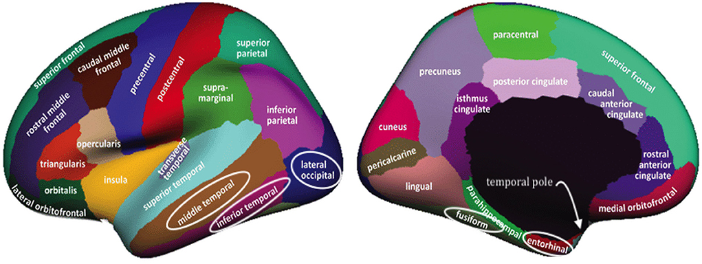
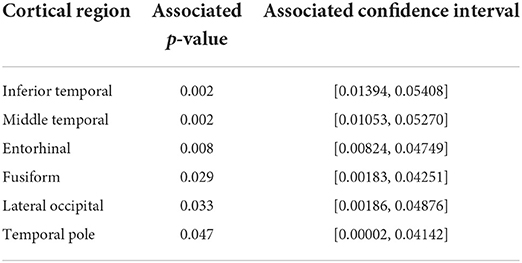
We indicated in the manuscript that the confidence intervals for each predictor are based on the univariable approximation using the bootstrap-based confidence intervals. disPEER estimates, when the geodesic distance is employed, imply the highest number of significant regions in relation to the other methods. Moreover, it turns out that the significantly associated areas are located close to each other on the cortical surface. Based on the disPEER estimates, we conclude that they may be involved in language comprehension. We marked these regions using white rectangles in Figure 9. Also, we summarized the significant regions in Table 3, where we included corresponding p-values computed for bootstrap results. Indeed, the literature (Blank et al., 2002; Fridriksson et al., 2015; Mesulam et al., 2015) states that some areas of the left hemisphere are associated with language comprehension. The so-called Wernicke's and Broca's areas are the two main zones commonly known for being associated with speech production. However, the location and functionality of these regions are still not fully established. In the literature, we also find many different studies that demonstrate that normal communicative speech is reliant on the left hemisphere regions that are distant from the classically defined language areas of Wernicke's and Broca's areas (Blank et al., 2002; Mesulam et al., 2015).

FIGURE 9

Figure 9. Desikan-Killiany parcellation (original image from Klein and Tourville, 2012) of the left hemisphere with significant regions indicated by white loops. Regions are visible from lateral and medial perspectives (left and right, respectively).

TABLE 3

Table 3. Cortical regions in the left hemisphere with corresponding bootstrap-obtained p-values and non-adjusted 95% confidence intervals (for geodesic distance).

4. Discussion

The complexity of the human brain was a primary factor driving the search for another source of information that could improve the study of the associations between the structural properties of the cortex and neurocognitive outcomes as manifested by improvement in the regression coefficient estimation. In our work, we provided an extension of the method developed in Karas et al. (2019) by incorporating a distance measure among cortical regions to provide additional information in the penalization specified in Equation (2).

We studied the performance of the coefficient estimation with the incorporation of the structural connectivity and spatial proximity, and as an evaluation measure, we examined the relative MSE of coefficients defined in Equation (11). In our simulation study, we used two types of the distance term—Euclidean and geodesic distance. Also, we assumed different impacts on model coefficients from both sources of information. We observed that independently of the parameter specification and assumptions we make for the distance or b distribution, in most cases, estimation benefits from the incorporation of the between-region distance information. There is a significant improvement in disPEER estimation in terms of not only rMSE but also bias. Regarding the bias-variance trade-off, it is clearly visible that while ridge regression has the smallest variance with the highest bias, at the same time, disPEER and riPEER keep balance between these measures, with a visible advantage of our distance-based method.

disPEER was applied to the real data collected by the Human Connectome Project. We studied a cognitive function of vocabulary comprehension and noticed that in the left hemisphere, disPEER estimation was driven mainly by the proximity and cortical regions chosen by this method were located adjacently. Moreover, these neighboring regions indicated as significant by disPEER were situated within the so-called Wernicke's and Broca's areas, which according to the literature are involved in language ability (see Blank et al., 2002; Fridriksson et al., 2015; Mesulam et al., 2015).

In our future work, we will explore utilizing sparsity-inducing penalties, e.g., LASSO (Tibshirani, 1996). We will also expand our predictor space to include the activation maps from the task-based fMRI studies with the penalties imposed by both spatial distance and structural connectivity matrices and we will incorporate the simulation-based approach of Ruppert et al. (2003) to establish simultaneous confidence intervals for all predictors.

Data availability statement

Publicly available datasets were analyzed in this study. This data can be found at: http://www.humanconnectomeproject.org/data/.

Ethics statement

Ethical review and approval was not required for the study on human participants in accordance with the local legislation and institutional requirements. The patients/participants provided their written informed consent to participate in this study.

Author contributions

AS and JH implemented the statistical model and its application to the synthetic and real data and created the first draft of the manuscript. TR, DB, and KP contributed to the theoretical part of the study and provided feedback for the paper. JH, KA, and JG processed the cortical data including calculation of the geodesic and Euclidean distance. All authors contributed to the manuscript revisions, read, and approved the submitted version.

Funding

This research was mainly conducted when AS was a Short-Term Visiting Research Scholar at the Indiana University School of Public Health-Bloomington on Exchange Visitor Program P-1-00104 in 2021. Partial support for this research was provided by the NIMH grant R01 MH108467 and by the NINDS grant R01 NS112303.

Acknowledgments

We would like to give our acknowledgment to Dr. Trosset for insightful discussions on the distance and proximity measures. Partial content of this work was also included in the Master's thesis which was defended at the University of Wroclaw with number of diploma 2097/2021 3.

Conflict of interest

The authors declare that the research was conducted in the absence of any commercial or financial relationships that could be construed as a potential conflict of interest.

Publisher's note

All claims expressed in this article are solely those of the authors and do not necessarily represent those of their affiliated organizations, or those of the publisher, the editors and the reviewers. Any product that may be evaluated in this article, or claim that may be made by its manufacturer, is not guaranteed or endorsed by the publisher.

Supplementary material

The Supplementary Material for this article can be found online at: https://www.frontiersin.org/articles/10.3389/fnins.2022.957282/full#supplementary-material

Footnotes References

Benning, M., and Burger, M. (2018). Modern regularization methods for inverse problems. Acta Numer. 27, 1–111. doi: 10.1017/S0962492918000016

CrossRef Full Text | Google Scholar

Bertero, M., Boccacci, P., and Koenig, A. (2001). Introduction to inverse problems in imaging. Opt. Photon. News 12, 46–47. doi: 10.1201/9781003032755

CrossRef Full Text | Google Scholar

Blank, S., Scott, S., Murphy, K., Warburton, E., and Wise, R. (2002). Speech production: Wernicke, Broca and beyond. Brain 125, 1829–1838. doi: 10.1093/brain/awf191

PubMed Abstract | CrossRef Full Text | Google Scholar

Brezinski, C., Redivo-Zaglia, M., Rodriguez, G., and Seatzu, S. (2003). Multi-parameter regularization techniques for ill-conditioned linear systems. Numer. Math. 94, 203–228. doi: 10.1007/s00211-002-0435-8

CrossRef Full Text | Google Scholar

Brzyski, D., Karas, M. M., Ances, B., Dzemidzic, M., Goni, J. W., Randolph, T., et al. (2021). Connectivity-informed adaptive regularization for generalized outcomes. Can. J. Stat. 49, 203–227. doi: 10.1002/cjs.11606