Linear leaky-integrate-and-fire neuron model based spiking neural networks and its mapping relationship to deep neural networks

and h ∈ represent the row and column of neuron, respectively. Considering that we use the frequency encoding, we integrate the input spike sequences in the time domain firstly. The number of spikes N of neuron nl, h is computed as: Nl,h=∫oTIl,h(t)dt (18)

where T is the time window. And the we adopt the neuron with the largest number of spikes in the time window as the output neuron of the max-pooling layer, shown in Figure 15.

FIGURE 15

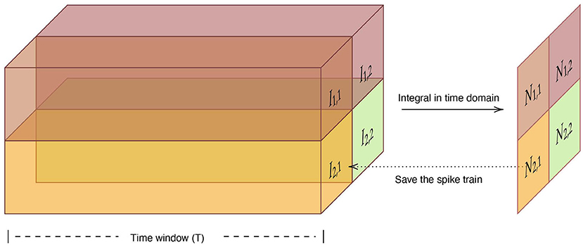
Figure 15. The structure and information flow of spiking max-pooling layer.

5.4.3. Datasets and implementation

We set a group of experiments based on MNIST and CIFAR-10 datasets. We convert the supervised-trained weights of CNN into an SNN with the same structure and verify the gap between CNN and SNN in the test dataset.

A ConvNet with two convolution layers (Conv.12 5 × 5 - Conv.64 5 × 5), ReLU activations, and two max-pooling layers are trained on the MNIST dataset. The structure of networks is the same as architectures used by authors in Diehl et al. (2015) and shown in Table 5. In the experiment, we select the best-performing model after the verification accuracy has converged, and directly transform it into LIF-SNN. The LIF-SNN uses frequency coding and sets the parameters of each Linear LIF neuron to be equivalent to the ReLU-AN model.

TABLE 5

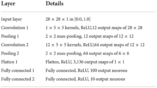
Table 5. CNN baseline model for MNIST dataset (with softmax output layer).

Verified by experiment, a shallow convolutional net can achieve high performance on the MNIST dataset. A more complex model should be performed to evaluate the equivalence in a deep structure. We use the AlexNet architecture (Krizhevsky et al., 2012) and VGG-16 (Simonyan and Zisserman, 2015) architecture for the CIFAR-10 dataset. In the simulation, we did not use image pre-processing and augmentation techniques and kept consistent with the AlexNet and VGG-16 model architecture. And all the CNNs in the experiment did not use bias. Because the conversion between bias and membrane conductance needs to limit the weight of the neural network, see Section 4.3 for details. The equivalence between neuron models with bias has been proved in the previous chapter through formulas and simulation experiments, see Section 5.2.

By verifying the similarity between CNN and LIF-SNN, we proved the equivalence of the Linear LIF model with the ReLU-AN model. However, we are not aiming at the highest performance of CNNs under supervised learning, so we don't use regular operations like image pre-processing, data augmentation, batch normalization, and dropout.

5.4.4. Experiments for ConvNet architectures

The network used for the MNIST dataset is trained for 100 epochs until the validation accuracy stabilizes, and achieves 98.5% test accuracy. For LIF-SNN, we set the time window of simulation as 2s and normalized values of the MNIST images to values between 0 and 10. Based on the algorithm of information coding, spike trains between 0 and 10 Hz were generated and presented to the LIF-SNN as inputs. The input trains are processed by convolutional layers and max-pooling layers, and finally are vectorized and fully connected to ten Linear LIF node as the output. We counted the number of spikes in output spike trains, used the node with the highest frequency as the output of LIF-SNN.

Figure 16 shows the comparison between ReLU-based ConvNet and LIF-SNN, and the confusion matrix. We use the number of spikes to represent the spike trains. The comparisons of feature maps between ReLU-based ConvNet and LIF-SNN are shown in the left figure in Figure 16. By comparing the upper and lower figures, we can obtain that the original images have undergone convolutional and pooling operations, which are the same as the information represented by spiking convolutional and spiking max-pooling operations after frequency encoding. Ideally, that is, the encoding time is infinite and the sampling frequency is infinite, the image in the bottom row should be the same as the image in the top row. The right figure in Figure 16 shows the confusion matrix of MNIST data, the actual labels are the outputs of CNN, and the predicted labels are the outputs converted LIF-SNN. We selected 2,000 sets of images from the test dataset for testing. Compared with the output of CNN, the accuracy of LIF-SNN reached 100%. Under the structure of the convolutional and pooling layers, the two neuron models can also maintain high behavioral equivalence. The experiments also proved the equivalence of the ReLU-AN model and the CLIF model in the convolutional neural network composed of convolutional and max-pooling layers.

FIGURE 16

Figure 16. Performance of SNN with ConvNet architecture. The left figure shows comparison of feature maps between ReLU-based ConvNet and LIF-SNN. The top figure shows the test image, feature map of convolutional layer, and feature map of max-pooling layer. The images in the bottom rows show the spikes count of output of LIF-SNN. The right figure shows the confusion matrix of LIF-SNN relative to the output of CNN.

5.4.5. Experiments for deep convolutional architectures

In this subsection, a more thorough evaluation using more complex models (e.g., VGG, AlexNet) and datasets (e.g., CIFAR that includes color images) are given. Since the main contribution of this work is establishing the mapping relationship and not in training a SOTA model. In the training of AlexNet and VGG-16 based on the CIFAR-10 dataset, we did not use data augmentation and any hyper-parameter optimization. Although the classification accuracy based on the existing training mechanism is not the best, it is already competitive.

The AlexNet architectures network with five convolutional layers, ReLU activation, 2 × 2 max-pooling layers after the 1st, 2nd, and 5th convolutional layer, followed by three fully connected layers was trained on the CIFAR-10 dataset. The AlexNet network is created based on PyTorch and trained on 2 GPUs with a batchsize of 128 for 200 epochs. Classification Cross-Entropy loss and SGD with momentum 0.9 and learning rate 0.001 are used for the loss function and optimizer. We selected the best-performance model and convert the weights to the LIF-SNN with same structure. The best validation accuracies (all the test data) of AlexNet for the CIFAR-10 dataset we achieved were about 80.23%. The simulation process is the same as the simulation of the MNIST dataset. Figure 17 shows the comparison of the feature map and the confusion matrix. Based on the equivalence of Linear LIF model and ReLU-AN model, the outputs of LIF-SNN are infinitely close to the outputs of CNN. Besides, in order to quantitatively analyze the equivalence of LIF-SNN and CNN after weight conversion, we compared the classification accuracy of the two models and drew a confusion matrix. We verified all the test samples and used the output of CNN as the label. LIF-SNN achieved 99.46% accuracy on the CIFAR-10 dataset.

FIGURE 17

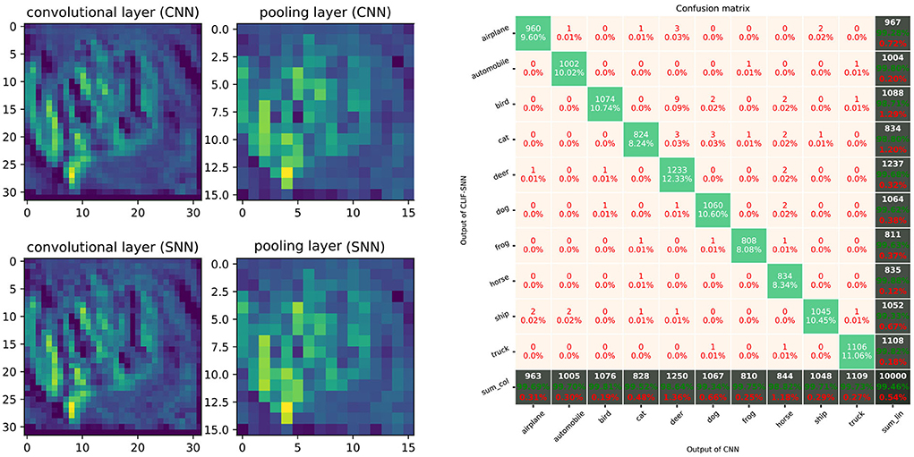
Figure 17. Performance of SNN with AlexNet architecture. The left part of figure shows the comparison of feature maps of convolutional layers and max-pooling layer between ReLU-based CNN and LIF-SNN with same input and connection weights. The right part of figure shows the confusion matrix for CIFAR-10 classification.

The experiment of the VGG-16 structure network is based on the proposal outlined by the authors in Sengupta et al. (2019). Sengupta made effort to generate an SNN with deep architecture and applied it to the VGG-16 network. Similarly, we trained a VGG-16 network based on the CIFAR-10 dataset. The best validation accuracy we achieved is about 88.58%. We only replace the ReLU-AN model with the Linear LIF model. For 800 images of the test dataset, LIF-SNN obtained a test accuracy rate of 99.88%, and the accuracy rate is calculated in the same way as Section 5.3.2. Besides, with the Spike-Norm proposed by Sengupta et al. (2019), the algorithm allows conversion of nearly arbitrary CNN architectures. The way to combine it with parameter mapping needs to be explored to minimize the accuracy loss in ANN-SNN conversion.

Table 6 summarizes the performance of converted LIF-SNN on MNIST and CIFAR-10 datasets. We list the results of some ANN-to-SNN works and compare them based on the error increment between CNN and SNN as an indicator. Error increment refers to the gap between the classification accuracies of ANN and SNN. At the same time, we also give the network structure and parameters for reference in Table 6. The transformation based on model equivalence achieved the best performance. For the shallow network, we can achieve error-free transformation, and for the deep network, we can minimize the error to 0.08%.

TABLE 6

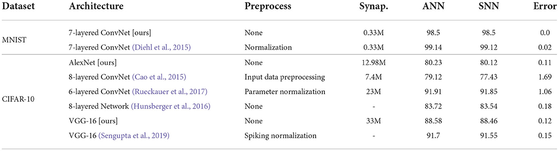
Table 6. Classification error rate on MNIST and CIFAR-10 dataset.

Through the simulation of neural networks with different structures, including shallow and deep networks, we proved the equivalence of the Linear LIF model and the ReLU-AN model. And it is verified that the conversion from CNN to SNN can also be completed in convolutional structures, deep networks, and complex data sets.

5.5. Error analysis

There is still a gap between the LIF/SNN and ReLU/DNN. We believe that the main reason for the error is that the ideal simulation conditions are not achieved. Under ideal conditions, we have infinite encoding time and infinite sampling frequency. However, considering the demand for computing power, our simulations are compromised between accuracy and computing power consumption. Besides, the mapping relationship we proposed is established under the condition that multiple inputs with the same frequency. While in more general conditions, there are still errors.

Here we explore the relationship between coding time and error. We define the output of the Linear LIF model as:

where N is the number of action potentials of spike train within the coding time, and T is the coding time. Then we assume that our expected output frequency is f, then:

Then the error between the expected output frequency and the true output frequency is:

|f-f′|=|f-NT|=|f-[f·T⌉T|<1T (21)

We explore the L2 norm as the error under the same frequency input condition. Figure 18 shows the relationship between simulation error and the theoretical error of LIF-AN. We can see that the actual error is consistent with the theoretical error trend, and we can reduce the error by increasing the encoding time. When the coding time is 10s, LIF-SNN achieves an error of less than 1% in the moto/face and MNIST data sets.

FIGURE 18

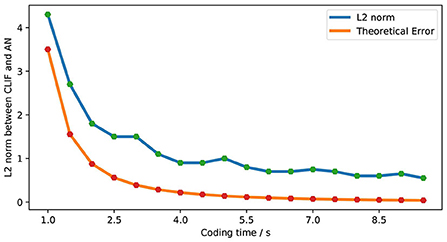
Figure 18. Comparison of theoretical error and actual error.

6. Conclusion and discussion 6.1. Brief summary

Despite the great successes of DNN in many practical applications, there are still shortcomings to be overcome. One way to overcome them is to look for inspiration from neuroscience, where SNNs have been proposed as a biologically more plausible alternative.

This paper aims to find an equivalence between LIF/SNN and ReLU/DNN. Based on a dynamic analysis of the Linear LIF model, a parameter mapping between the biological neuron model and the artificial neuron model was established. We analyzed the equivalence of the two models from the aspects of weight, bias, and slop of activation function, and verified it both theoretically and experimentally, from a single neuron simulation to a neural network simulation. It shows that such an equivalence can be established, both the structural equivalence and behavioral equivalence, and the Linear LIF model can complete the information integration and the information processing of the linear rectification.

This mapping is helpful for the combination of an SNN with an artificial neural network and increasing the biological interpretability of an artificial neural network. It is the first step toward answering the question of how to design more causal neuron models for future neural networks. Many scholars believe that interpretability is the key to a new artificial intelligence revolution.

At the same time, the equivalence relationship is the bridge between machine intelligence and brain intelligence. Exploring new neuron models is still of great importance in areas such as unsupervised learning. As brain scientists and cognitive neuroscientists unravel the mysteries of the brain, the field of machine learning will surely benefit from it. Modern deep learning takes its inspiration from many areas, and it makes sense to understand the structure of the brain and how it works at an algorithmic level.

6.2. Future opportunities

The architecture of SNN is still limited to the structure of DNN. Compared with DNN, SNN only has the synaptic connection weights which can be trained, while the weights, bias and activation function (dynamic ReLU, Microsoft Chen et al., 2020) can be trained in DNN. Therefore, we expect Linear LIF model and the parameter mapping relationship can bring innovation to SNN fromthose aspects.

6.2.1. A new way to convert ANN to SNN

With the new approach of converting pre-trained ANN to SNN, we will have a better expression of bias in SNN. Most conversion methods restrict the structure of ANN and directly map the weight. However, bias is also an important parameter in the deep learning network, and we can convert bias into membrane conductance gl based on parameter mapping relationship. In this way, SNN and ANN can maintain high consistency and improve the effect of some tasks. Especially in the convolutional neural network, the connectable region of neurons is small, which is more conducive to the conversion of bias into the parameters in the Linear LIF model.

6.2.2. Parameters training of linear LIF model

All the parameters of LIF model can be trained or transformed, which is the fundamental difference from other SNN. Based on the parameters mapping relationship, we can map the trained parameters of DNN to the biological parameters of LIF model, to ensure that each node in SNN has its own unique dynamic properties. At the same time, we know the meaning of each parameter, and we can also carry out the direct training of parameters. In biology, it is also worth investigating whether other parameters of neurons, besides weights, will change.

6.2.3. Dynamic activation function

As the number of layers in the network increases, the number of spikes decreases. We generally adjust the spiking threshold to solve this problem. But we know that the shape of the action potential is essentially fixed, and the spiking threshold of neurons does not change. The membrane capacitance represents the ability to store ions, that is, the opening and closing of ion channels. So, when the number of spikes is low, we can reduce the membrane capacitance and increase the membrane capacitance instead. In parameter mapping, it is similar to dynamic ReLU.

Data availability statement

The original contributions presented in the study are included in the article/Supplementary material, further inquiries can be directed to the corresponding author.

Author contributions

FX conceived the original idea. SL and FX conducted the theoretical derivation and algorithmic development, contributed to the development of the concepts, the analysis of the data, and the writing of the manuscript. Both authors contributed to the article and approved the submitted version.

Funding

This work has been supported by National Natural Science Foundation of China (Grant No. 61991422 to FX).

Conflict of interest

The authors declare that the research was conducted in the absence of any commercial or financial relationships that could be construed as a potential conflict of interest.

Publisher's note

All claims expressed in this article are solely those of the authors and do not necessarily represent those of their affiliated organizations, or those of the publisher, the editors and the reviewers. Any product that may be evaluated in this article, or claim that may be made by its manufacturer, is not guaranteed or endorsed by the publisher.

Supplementary material

The Supplementary Material for this article can be found online at: https://www.frontiersin.org/articles/10.3389/fnins.2022.857513/full#supplementary-material

References

Bear, M. F., Connors, B. W., and Paradiso, M. A. (2007). Neuroscience - Exploring the Brain. 3rd Edn. Baltimore, MD: Lippincott Williams & Wilkins.

More from this channel

Linear leaky-integrate-and-fire neuron model based spiking neural networks and its mapping relationship to deep neural networks

留言 (0)