1 Introduction

Autism spectrum disorder (ASD) is a series of complex neurodevelopmental disorders that may affect a patient’s social, behavioral, and communication abilities (Molnar-Szakacs et al., 2021). According to the Global Burden of Disease Study in 2019, there are approximately 28 million ASD patients worldwide (Vos et al., 2020). ASD is more common in children; however, few reports of cases in adults are found due to the lack of effective intervention or unfortunate experience in adulthood. The traditional diagnosis of ASD is mainly based on the observations of doctors and various rating scales. According to the Diagnostic and Statistical Manual of Mental Disorders, Fourth Edition (DSM-IV) (American Psychological Association, 1994), ASD can be divided into multiple subtypes, including autism, Asperger’s, pervasive developmental disorder not otherwise specified (PDD-NOS), Rett’s disorder, and childhood disintegrative disorder. However, in the Diagnostic and Statistical Manual of Mental Disorders, Fifth Edition (DSM-5) (American Psychiatric Association, 2013), Rett’s disorder and childhood disintegrative disorder are no longer considered subtypes of ASD (Oberman and Kaufmann, 2020). Regardless of the rating scale used, it is widely recognized that ASD has multiple subtypes, and disorders including autism, Asperger’s, and PDD-NOS are the basic subtypes of ASD (Brown et al., 2010; Tamura et al., 2010; Sharma et al., 2018). The basis of traditional diagnosis is to compare the behavior of a person with the typical performance described in the checklist. In other words, the experience of the doctor, rather than the biological signals of the patient, plays an important role in the diagnosis. Therefore, traditional diagnoses based on rating scales are likely to be affected by various subjective factors. This subjectivity may lead to misdiagnosis, considering the heterogeneity among patients and differences between subtypes.

With the development of medical technology, many non-invasive acquisition methods have emerged to obtain signals from the human brain, including electroencephalography (EEG), magnetic resonance imaging (MRI), and functional MRI (fMRI). These non-invasive acquisition methods provide new ideas for the study of ASD (Tuchman and Rapin, 2002; Wang et al., 2013; Pierce et al., 2021). In recent years, many ASD studies have been conducted based on fMRI, due to its capabilities of providing a type of four-dimensional data that contains spatial and temporal information of the whole brain. Some studies have attempted to illustrate the impairment in brain function of ASD patients through fMRI analysis. Haghighat et al. found differences in between-connectivity among default mode network, salience-executive network, and fronto-parietal network between ASD and healthy children (Haghighat et al., 2021). Maximo et al. observed reduced brain entropy in the prefrontal areas of children with autism (Maximo et al., 2021). Another part of the studies tried to apply the deep learning method to fMRI data and classify ASD patients and healthy controls. A long short-term memory model was proposed in 2019 with data from four sites, achieving an average accuracy of 74.8% (Dvornek et al., 2019). Soon after, a 3D convolutional neural network (CNN) was proposed in 2020 and achieved an accuracy of 66.0% with data from 2085 subjects (Thomas et al., 2020). Some new deep learning methods including graph convolutional network have also appeared in the ASD studies (Parisot et al., 2018). In addition to the functional characteristics, there have also been studies focusing on the differences in brain structure between patients with ASD and healthy controls. Yaxu et al. observed atypical development in gray matter volume (GMV) and gray matter density (Yaxu et al., 2020). Watanabe and Rees identified age-associated atypical increases in relative GMVs of the regions of auditory and visual networks and an age-related aberrant decrease in the relative GMV of the fronto-parietal network in children with ASD (Watanabe and Rees, 2016). In addition, GMV is an important feature of ASD classification (Arya et al., 2020).

Although many studies have focused on the analysis or classification of ASD, few have focused on its subtypes. Previous studies have tended to focus on the difference between single subtype and typically developing controls or other mental disorders, such as attention deficit hyperactivity disorder and schizophrenia (Chen et al., 2017; Huang et al., 2020; Shi et al., 2020). In this study, we focused on the functional and structural differences between the three common ASD subtypes: autism, Asperger’s, and PDD-NOS. For fMRI data, we applied a tensor decomposition method to capture the different brain communities in the ASD subtypes. In recent years, tensor decomposition has been used to extract the features of brain activity from fMRI data (Aggarwal and Gupta, 2019; Li et al., 2020). Resting-state fMRI dataset is a high dimension data which is a combination of brain regions, time and patients. Tensor decomposition is a good tool to extract a compressed feature set or to alleviate the joint effect of factors to analyze a certain dimension. As additional functional features, amplitude of low-frequency fluctuation (ALFF) (Wang Z. et al., 2019; Arya et al., 2020) and fractional ALFF (fALFF) (Zou et al., 2008; Itahashi et al., 2015) of the subtypes, were extracted from fMRI data, and as a representation of structural features, the gray matter volume (GMV) (Zhao et al., 2022) was extracted to evaluate the variation of the brain structures among the subtypes. Based on the three functional and one structural brain features, we aimed to provide a systematic understanding of the heterogeneity among the three subtypes, which may provide a new idea for the discrimination of ASD subtypes.

2 Materials and methods

In this study, we extracted four types of brain features, three functional and one structural features to discover the differences between the ASD subtypes as summarized in Figure 1A. As the first functional feature, we presented a brain pattern extraction method to determine the brain patterns and related sub-networks of different ASD subtypes. For the other two functional features, we extracted two common features, amplitude of low-frequency fluctuation (ALFF) and fractional ALFF (fALFF). Finally, for the structural feature, we extracted gray matter volume (GMV) to examine whether there are structural changes between the subtypes. In this section, we first introduce the fMRI dataset used in this study (Section 2.1). Then, we introduce the fundamental features used in this study (Section 2.2), including functional connectivity (FC), ALFF, fALFF, and GMV. As shown in Figure 1B, we proposed a tensor-decomposition-based brain pattern feature extraction method for the ASD subtypes to show brain community features (Section 2.3). Finally, we use a statistical test to check whether there are significant differences between the ASD subtypes in terms of functional and structural features (Section 2.4).

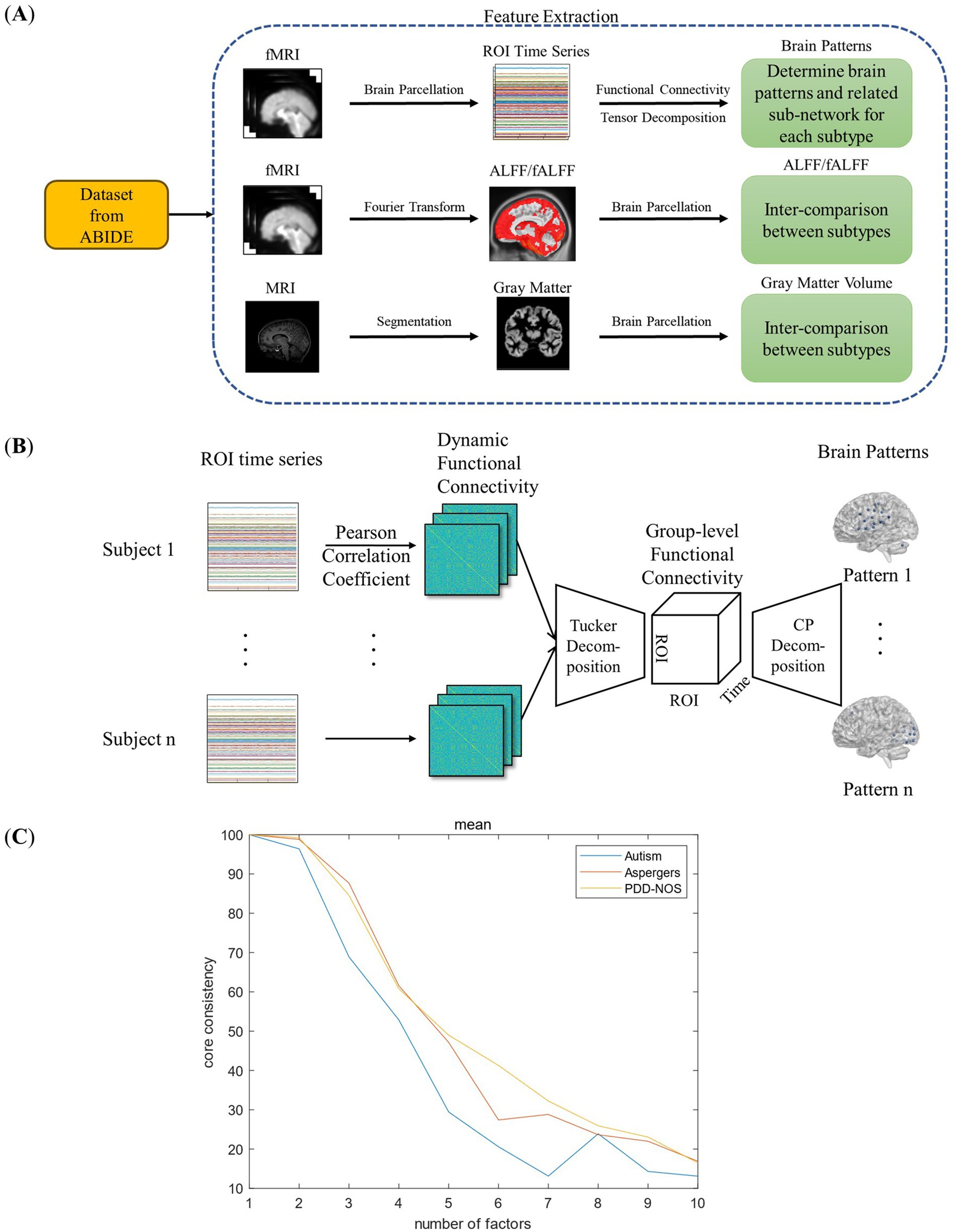
Figure 1. Framework of this study: (A) feature extraction process. (B) Framework of the FC-based brain pattern feature extraction. (C) Detection of the number of the brain patterns.

2.1 Data acquisition

The fMRI dataset used in this study was obtained from the Autism Brain Imaging Data Exchange I (ABIDE I) (Craddock et al., 2013; Di Martino et al., 2014), a public dataset involving resting-state fMRI and anatomical and phenotypic datasets from 17 international sites. Full details for acquisition parameters, site-specific protocols and descriptions about the participants can be found at https://fcon_1000.projects.nitrc.org/indi/abide/abide_I.html. The entire dataset contains data from 539 patients with ASD and 573 typical controls. However, since our work focused on the differences between ASD subtypes, only resting-state fMRI data and anatomical data from patients with ASD subtypes were considered for extracting functional and structural features, respectively. The inclusion criteria were as follows.

• With exact subtype label

• Without data error

• Without long-time fixed signal

The first two inclusion criteria were based on phenotypic data from the ABIDE I dataset. In terms of the third one, because it is based on the functional connectivity method, for the completeness of the article, the inclusion criteria will be described in Section 2.2.

The corresponding datasets used in this study are described in Table 1. The dataset contained resting-state fMRI and anatomical data from 152 patients with autism, 54 patients with Asperger’s, and 28 patients with Pervasive Developmental Disorder-Not Otherwise Specified (PDD-NOS). The labels of the subtypes are from the phenotypic data provided by the ABIDE project. The diagnosis of different subtypes and detailed information of the subjects are provided in the Supplementary material. To make our results more robust, we used the same preprocessed data from the ABIDE Preprocessed project (Craddock et al., 2013) with the pipeline provided by the Connectome Computation System (CCS) (Xu et al., 2015). The steps and parameters of the CCS pipeline are presented in Table 2. In this study, the fMRI data were collected using the filt_global preprocessing strategy with band-pass filtering (0.01–0.1 Hz) and global signal regression. Registration from the original to Montreal Neurological Institute’s 152 (MNI152) brain template was calculated using a combination of linear and non-linear transforms.

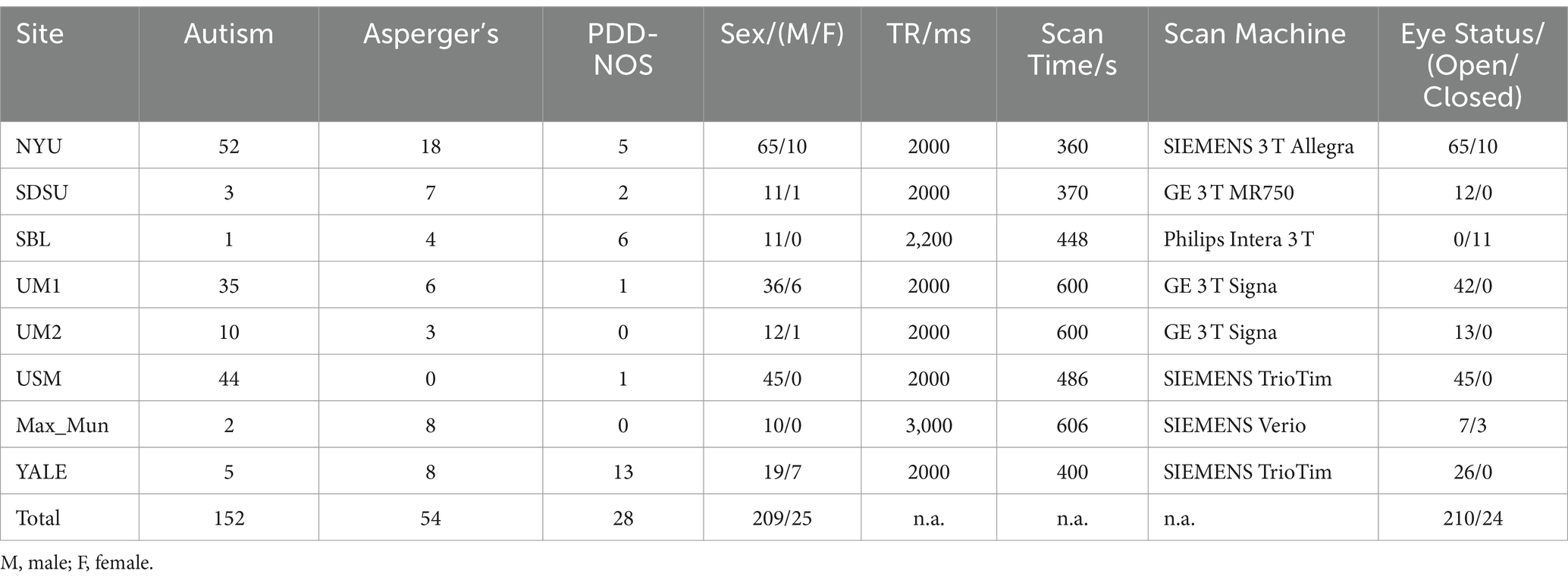
Table 1. Details of fMRI data from ABIDE I used in this study.

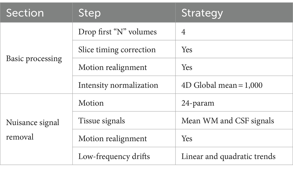
Table 2. The steps and parameters in the CCS pipeline.

2.2 Feature extraction 2.2.1 Brain atlas

Based on the anatomical MRI and resting-state fMRI analysis, regions of interest (ROI) based features and brain networks features are extracted and analyzed to provide some significant information for the ASD subtypes discrimination. The brain data ROIs, which are defined by brain atlases, represent the averages of the values from the brain regions (voxels) with similar functions. Brain networks are even bigger concepts representing sets of different ROIs that work together to achieve higher-level cognitive functions. In this study, Craddock 200 brain parcellation (Craddock et al., 2012) was selected to obtain the ROI-based features for its data-driven nature. The Craddock 200 atlas is a gray matter mask that contains 200 ROIs, which can provide sufficient regions to discover the differences in functional and structural features. The robust performance of the atlas has also been verified in several previous studies (Liang and Xu, 2022; Kunda et al., 2023).

In terms of large-scale brain networks, this study performed an analysis on the 12 well-defined brain sub-networks provided by Power et al. (2011). To incorporate these sub-networks into the Craddock 200 atlas, we chose the adopted sub-networks provided by Ingalhalikar et al. (2021). The original networks were assigned to the Craddock 200 atlas after matching each ROI from the Craddock 200 atlas with the ROI from the Power264 atlas, based on the minimum Euclidean distance.

2.2.2 Functional connectivity

Functional connectivity (FC) is an effective method for evaluating the relationships between different brain regions. FC is a common fMRI feature that numerous studies have used to identify the unique characteristics of the disease. According to the length of the time duration that is considered, FC can be divided into static and dynamic FC. Static FC evaluates the relationships between ROIs over the entire time length, while dynamic FC evaluates such relationships based on multiple time windows. Previous studies have shown that FC may have different patterns during the scan period in resting-state fMRI data from patients with ASD (Yao et al., 2016; Aggarwal and Gupta, 2019). Therefore, in this study, the dynamic FCs of each patient were extracted to evaluate the various patterns of the subtypes.

Dynamic FC was calculated based on the ROI signals in the sliding windows. Denote the time length of the sliding window is L , the TR of site i is TRi , then the signal length Ni for the time window can be defined as Equation 1:

The length of the time window L is not chosen subjectively either. Leonardi and Van De Ville found that the length selection of the sliding window is related to the low-end cutoff frequency of the bandpass filter used in data processing (Leonardi and Van De Ville, 2015):

flow in Equation 2 is the low-end cutoff frequency of the bandpass filter. In this study, the bandpass filter used in the preprocessing was 0.01 ~ 0.1 Hz, thus making the length of the time window L 100 s.

After determining the length of the sliding window, the FC in each time window can be described as a matrix of Pearson correlation coefficients between each two ROIs:

ρX,Y=covXYσXσY=EX−μXY−μYσXσY    (3)

ρX,Yis the Pearson correlation coefficient between ROI X and ROI Y in the time window. μis the mean value of the ROI signal in the time window and σ is the standard deviation of the ROI signal in the time window. The range of ρX,Yis −1≤ρX,Y≤1 , which represents the relationship between the two ROIs in the time window.

In addition to evaluating the relationship between ROIs, dynamic FC can also be used to check the quality of the data. As described in Section 2.1, dynamic FC was also used for the automatic selection of resting-state fMRI data. In the calculation of the dynamic FC, we sometimes found errors in the results. From Equation 3, we know that there will be an error in the calculation only when the standard deviation of the ROI signal is zero. In other words, when errors were found, at least one of the ROI signals remained unchanged during the time window. In fact, when we rechecked the original time series data, we found that some of the patient data had constant ROI signals. Therefore, in this study, dynamic FC was also used for the quality control of the data. When there was an error in the calculation, we excluded the data of the corresponding patients from the dataset (data from 15 subjects were excluded).

Finally, after calculating the dynamic FC, the FCs from patients with different ASD subtypes were grouped. However, as can be seen from Table 1, different sites had different scan times. Therefore, to facilitate subsequent processing, the data length of the dynamic FC was set to 120.

2.2.3 Frequency domain features

In addition to the dynamic FC extracted from the ROI signal, which is a temporal feature based on resting-state fMRI data, we also utilized spectral features to determine the differences between ASD subtypes. In previous studies, low-frequency fluctuations in resting-state fMRI data have been proven to effectively reflect the brain activity of a subject during the scanning process (Zang et al., 2007; Hu et al., 2014). Therefore, the spectral features, ALFF and fALFF, were extracted to investigate the differences of the ROIs in each subtype.

ALFF aims to directly examine the low-frequency of each voxel. The ALFF value is defined as the average amplitude from each frequency point in the low-frequency band. To make it clear, for the time signal of voxel x , the signal yt after bandpass-filtering can be described as Equation 4:

yt=∫0+∞xτ·ht−τdτ    (4)

where ht denotes the bandpass filter. Note the power spectrum of yt as Yf , then the ALFF value of voxel x can be described as Equation 5:

ALFFx=∫flowfhighYfdffhigh−flow    (5)

where fhigh is the high-end cutoff frequency, and flow is the low-end cutoff frequency. To be consistent with the ALFF features used in previous studies, the ALFF map used in this work is also from the CCS pipeline in the ABIDE Preprocessed project. Before extracting the ROI-level ALFF features, we normalized the ALFF map of each patient using the z-score method. Finally, the average of the ALFF values from the voxels belonging to the same ROI were calculated.

fALFF is also a common spectral feature in fMRI studies. In contrast to ALFF, fALFF also considers the signal of the non-filtered data. For the time signal of voxel x , note Xfilteredf as the power spectrum after bandpass filtering and Xnon−filteredf as the power spectrum of non-filtered data. The fALFF value of voxel x can be described as Equation 6:

fALFFx=∫flowfhighXfilteredfdf∫0+∞Xnon−filteredfdf    (6)

where fhigh is the high-end cutoff frequency, and flow is the low-end cutoff frequency. Similar to the condition in ALFF, the fALFF map is also from the CCS pipeline in the ABIDE Preprocessed project. The same normalization and ROI-level feature extraction were implemented for the fALFF extraction.

2.2.4 Gray matter volume

As pointed out in previous studies, complicated functional changes or impairments occur in patients with ASD (Haghighat et al., 2021; Yang et al., 2023). Whether there are corresponding structural changes in the brain lobes or gyri remains a hot topic in research. In our study, GMV was extracted as a representation of structural features to determine whether changes in gray matter were similar to those in brain function. As mentioned in Section 2.1, the original MRI images used in this study were obtained from ABIDE anatomical data. To obtain the volume of each ROI, we used the Computational Anatomy Toolbox (CAT12) (Gaser et al., 2024) of the Statistical Parametric Mapping (SPM12) software (Ashburner, 2012) to perform the gray matter segmentation and ROI-level GMV estimation. In addition, z-score normalization was also adopted to compare the GMV of each ROI. To maintain consistency with the comparison above, the Craddock 200 atlas was used in the GMV calculation.

2.3 FC-based brain pattern extraction

Tensor decomposition is an effective method for separating attribute information from high-dimensional data. For the dynamic FC data in this study, which are composed of information on subtype, patient, ROI, and time, it is appropriate to use the tensor decomposition method to extract the brain patterns for each subtype. Previous studies have proven the effectiveness of tensor decomposition in brain data analysis (Becker et al., 2014; Aggarwal and Gupta, 2019; Zheng et al., 2021). Aggarwal et al. proposed an overlapping network identification method for multivariate vector regression-based connectivity (MVRC) based on tensor decomposition to determine the differences between patients with ASD and typical controls (Aggarwal and Gupta, 2019). However, the calculation of MVRC is complex, and the selection of the regularization parameters is empirical. In this study, we chose to use dynamic FC to perform brain pattern extraction for simplicity and objectivity. The framework for the brain pattern extraction is shown in Figure 1B.

2.3.1 Group-level dynamic FC

As shown in Figure 1B, before extracting the brain patterns, a group-level dynamic FC for each ASD subtype should be produced to represent the overall characteristics of the dynamic FC within the same subtype. Generally, such group-level FC is generated by simply averaging all FC matrices across patients, which is common and easy to realize. However, simply averaging assumes that all the patients’ data have the same contribution to the construction of group-level FC, which may introduce additional noise and ignore the heterogeneity among the patients of the same subtype. To address this issue, Tucker decomposition (Tucker, 1966) was implemented to calculate the weights for each patient’s data and construct a group-level dynamic FC (Figure 1B).

For the dataset of a single ASD subtype, the FC matrices of the subjects in each time window can form a three-order tensor. In this study, the group-level dynamic FC was calculated based on these tensors. Note the three-order tensor for one time window as T∈ℝN×N×S , where N is the number of ROIs, and S is the number of subjects. To obtain the group-level FC for each time point, Tucker decomposition was used to calculate the weight of the FC for each subject. The decomposition can be described as Equation 7:

T≈K×1X×2Y×3Z    (7)

where Kis the core tensor of the decomposition. Because we do not need to compress or approximate the FC data, the dimensions of the core tensor can be set to be the same as those of T , i.e., K∈ℝN×N×S . Besides, X∈ℝN×N , Y∈ℝN×N , Z∈ℝS×S are the orthonormal factor matrices along each mode of the tensor T , which contain the information of the corresponding attribute. And ×n is the mode n product in the decomposition. Obviously, only the matrix Z contains the information of the subjects, and from the principle of Tucker decomposition, the first column of Z contains the most significant FC features across the subjects. Therefore, in this study, Z1∈ℝS×1 as the first column of Z , is used as the weight to construct the group-level FC:

G¯=∑s=1SZ1sMs∑s=1SZ1s    (8)

In Equation 8, G¯∈ℝN×N is the group-level FC for the time point, and M is the FC matrix of the subject. A group-level dynamic FC tensor G∈ℝN×N×W can be constructed by calculating group-level FC at each time point, where W is the number of time windows.

2.3.2 Extraction of brain patterns

Brain patterns are sets of brain regions that can provide important community information during brain activity. The investigation of brain patterns may further illustrate the impairment in brain function based on FC. Previous studies have shown that non-negative tensor factorization has a good ability to extract pattern information from brain data (Ponce-Alvarez et al., 2015; Aggarwal and Gupta, 2019). In this study, we performed non-negative CANDECOMP/PARAFAC (CP) decomposition with adaptation of the block principal pivoting algorithm (Kim and Park, 2008) to extract multiple brain patterns of the subtypes.

Because we are performing non-negative CP decomposition, the absolute values of all group-level dynamic FCs of the subtypes are obtained. For convenience, the following group-level dynamic FCs refer to the absolute values. Given a fixed rank R , for the group-level FC tensor G∈ℝN×N×W , the decomposition of brain patterns can be described as Equation 9:

G≈∑i=1Rλixi∘yi∘zi    (9)

where “ ∘ ” is the sign of outer product, xi∈ℝN×1 , yi∈ℝN×1 and zi∈ℝW×1 are the factor vectors with the column norm of 1, which contains the information of the dimensions or modes of the tensor G . λi∈ℝ are the weights of the rank-one tensors which are produces by the outer product of xi , yi and zi . From the process of CP decomposition, we can know that xi and yi represent the information of the ROIs and the vector zi represents the information hidden in the time. Since the FCs are symmetric, the vectors xi and yi should be identical. Then, if we consider each rank-one tensor as a brain pattern, the rank R is actually the number of brain patterns hidden in the group-level FC tensor and xi or yi is actually the strength of the ROI in the corresponding pattern. Therefore, to determine the ROI communities in each brain pattern, we used the mean plus one standard deviation as the threshold value to detect ROIs with a high activity strength in the pattern.

2.3.3 Determination of the number of brain patterns

From the CP decomposition introduced in Section 2.3.2, we can know that rank R is actually the number of rank-one tensors. In other words, rank R determines the number of brain patterns in this study. However, the prediction of rank R in CP decomposition is an NP-hard problem. Various studies have proposed methods for determining the appropriate R for CP decomposition. In this study, we introduced the core-consistency method (Gauvin et al., 2014) for the prediction of rank R for its simplicity and efficiency.

For Tucker decomposition, the result is composed of factor matrices related to the corresponding dimensions of the tensor. Therefore, if the process is rewritten in the form of vectors, Tucker decomposition can be expressed as Equation 10:

T≈∑iX=1IX∑iY=1IY∑iZ=1IZkiXiYiZxiX∘yiY∘ziZ    (10)

where xiX , yiY , and ziZ are the columns of the original factor matrices X , Y and Z , respectively. kiXiYiZ is the element of the kernel tensor K . Comparing (9) and (10), we can find that when the kernel tensor K is a superdiagonal tensor, Tucker decomposition degenerates into CP decomposition. This implies that CP decomposition is a special form of Tucker decomposition. Then, for the fixed vectors xi , yi and zi of the CP decomposition (without the constraint that column is 1), with an appropriate rank R, the core tensor in Tucker decomposition should be similar to the superdiagonal tensor of ones. Thus, core consistency can be calculated as Equation 11:

coreconsistency=100×1−∑i=1R∑j=1R∑k=1Rkijk−12R    (11)

where kijk is the element in the Tucker decomposition. In this study, we calculated the core-consistency value from R=1 to R=10 to find the appropriate R value, and to ensure the reproducibility of the results, 3-fold cross-validation method was implemented. The results are shown in Figure 1C. As shown in Figure 1C, the core consistency values of the three ASD subtypes varied from R = 1 to R = 10, and we found a rapid decrease from R = 2 to R = 7. The research of Rasmus Bro et al. found that a core consistency value in the neighborhood of 50% leads to a problematic model (Bro and Kiers, 2003). Therefore, in this study, to find as many brain patterns as possible while ensuring the stability of the result, 60% is considered as an appropriate threshold, and the corresponding R values with the core consistency above the threshold are considered as the optimal number of brain patterns for each ASD subtype. As a result, the R values for autism were 3, and for Asperger’s and PDD-NOS were 4.

2.4 Statistical test

In this study, in addition to the comparison of brain patterns, we aimed to determine the differences between ASD subtypes by inter-comparison. To achieve this goal, the functional and structural feature values including ALFF, fALFF, and GMV of each ROI from different subtypes were compared by t-test to determine the differences between the subtypes. Furthermore, to discover such differences on a larger scale, we used the 12 well-defined brain networks parcellation to check the sub-networks that were involved in the comparisons. Because these comparisons involve multiple testing, in this work, the false discovery rate (FDR) correction was used for multiple testing correction. In addition, to check which ROIs were involved in all these comparisons (brain pattern, ALFF, fALFF, and GMV), we compared all the comparisons results and selected the overlapping ROIs. It should be noted here that for the comparison of brain patterns of the subtypes, a ROI was counted as involved in the comparison of one brain pattern if it appeared in one subtype and did not appear in the other.

3 Results

In this section, we present the results of the tensor decomposition-based brain pattern extraction and compare the functional and structural features. The brain patterns of each ASD subtype are described in Section 3.1. The inter-comparisons of ALFF, fALFF, and GMV between the subtypes are shown in Section 3.2. It should be noted that all the results from the comparisons based on the t-test in this study were at a significance level of 0.05, and FDR correction was adopted for multiple testing correction.

3.1 Brain pattern extraction

Figure 2 shows the brain patterns of each ASD subtype. Based on the results of the core consistency analysis as shown in Figure 1C, the number of brain patterns differed depending on subtypes. The patient group with autism tended to have three different brain patterns, while the patient groups with Asperger’s and PDD-NOS tended to have four different brain patterns. To clearly show the spatial distribution of the ROIs of the brain patterns, we projected the nodes onto a standard brain template using the BrainNet Viewer toolbox (Xia et al., 2013). As shown in Figure 2, the brain patterns extracted by the tensor decomposition method show a high degree of organization.

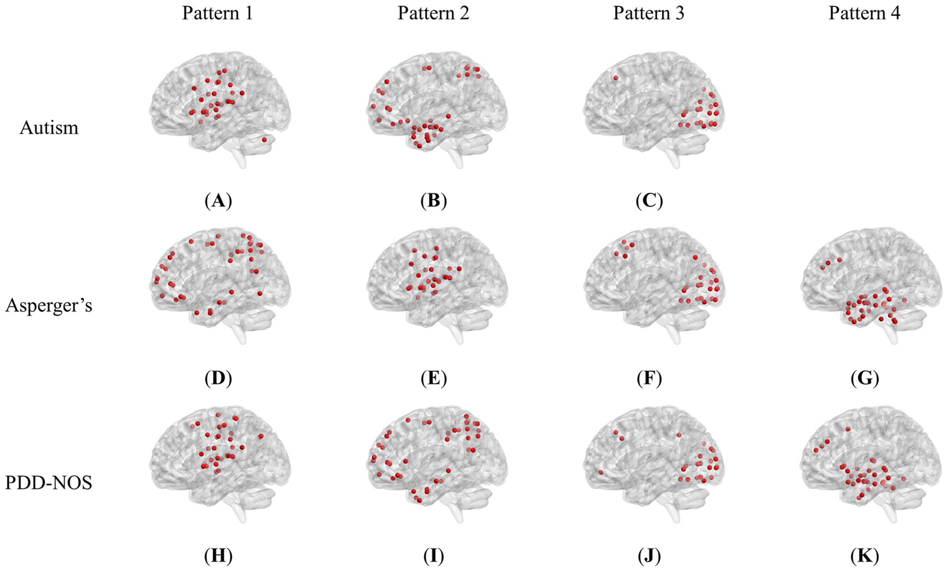
Figure 2. Brain patterns of the ASD subtypes: (A) Pattern 1 of autism (dominated by AN and CON). (B) Pattern 2 of autism (dominated by DMN and DAN). (C) Pattern 3 of autism (dominated by VN). (D) Pattern 1 of Asperger’s (dominated by DMN and DAN). (E) Pattern 2 of Asperger’s (dominated by AN and CON). (F) Pattern 3 of Asperger’s (dominated by VN). (G) Pattern 4 of Asperger’s (dominated by SCN and DMN). (H) Pattern 1 of PDD-NOS (dominated by AN, SMH and CON). (I) Pattern 2 of PDD-NOS (dominated by DMN and DAN). (J) Pattern 3 of PDD-NOS (dominated by VN). (K) Pattern 4 of PDD-NOS (dominated by SCN and DMN). AN, auditory network; CON, cingulo-opercular network; SCN, subcortical network; SMM, sensory/somatomotor mouth; SMH, sensory/somatomotor hand; SAN, salience network; FPN, fronto-parietal network; DMN, default mode network; DAN, dorsal attention network; VN, visual network; VAN, ventral attention network; CPN, cingulo-parietal network.

To demonstrate how these functional networks vary among subtypes, we followed the strategy adopted by Ingalhalikar et al. (2021) to divide the ROIs into 12 well-defined sub-networks based on different brain functions, including sensory/somatomotor hand (SMH), sensory/somatomotor mouth (SMM), cingulo-opercular network (CON), auditory network (AN), default mode network (DMN), cingulo-parietal network (CPN), visual network (VN), fronto-parietal network (FPN), salience network (SAN), subcortical network (SCN), ventral attention network (VAN), and dorsal attention network (DAN). Table 3 shows the sub-networks involved in different brain patterns and the number of ROIs that belong to the sub-networks (sub-networks with only one ROI are not listed). From Table 3, we can see that if we consider the sub-networks with more than five ROIs as the dominant sub-network in the brain pattern, we can find that some of the brain patterns of different subtypes can be grouped together. Pattern 1 of autism, Pattern 2 of Asperger’s and Pattern 1 of PDD-NOS can be gathered as Group 1, Pattern 2 of autism, Pattern 1 of Asperger’s and Pattern 2 of PDD-NOS can be gathered as Group 2, Pattern 3 of the three subtypes can be gathered as Group 3, and finally Pattern 4 of Asperger’s and PDD-NOS can be gathered as Group 4. We found that the sub-networks of Group 1 were mainly AN and CON, which were related to auditory activity, tonic alertness, and task control, while Pattern 1 of PDD-NOS showed a difference in SMH, which is linked to the motor activity of the hands. Group 2 mainly included the ROIs from the DMN and DAN, which are related to resting-state activity and task attention. Previous studies have pointed out that the activity of areas from the DMN is anti-correlated with that of the DAN regions (Wang J. et al., 2019; Qian et al., 2020). In this study, since we analyzed the brain patterns extracted by the non-negative CP decomposition, these two sub-networks were gathered in the same pattern, which is consistent with previous studies. Group 3 is mainly correlated with the VN, which is from Pattern 3 of all subtypes. Finally, Group 4 only included the brain patterns of Asperger’s and PDD-NOS, which are the patterns containing the ROIs from the SCN and DMN. Abnormalities in the FC of the SCN and DMN may lead to the main difference between autism and the other subtypes.

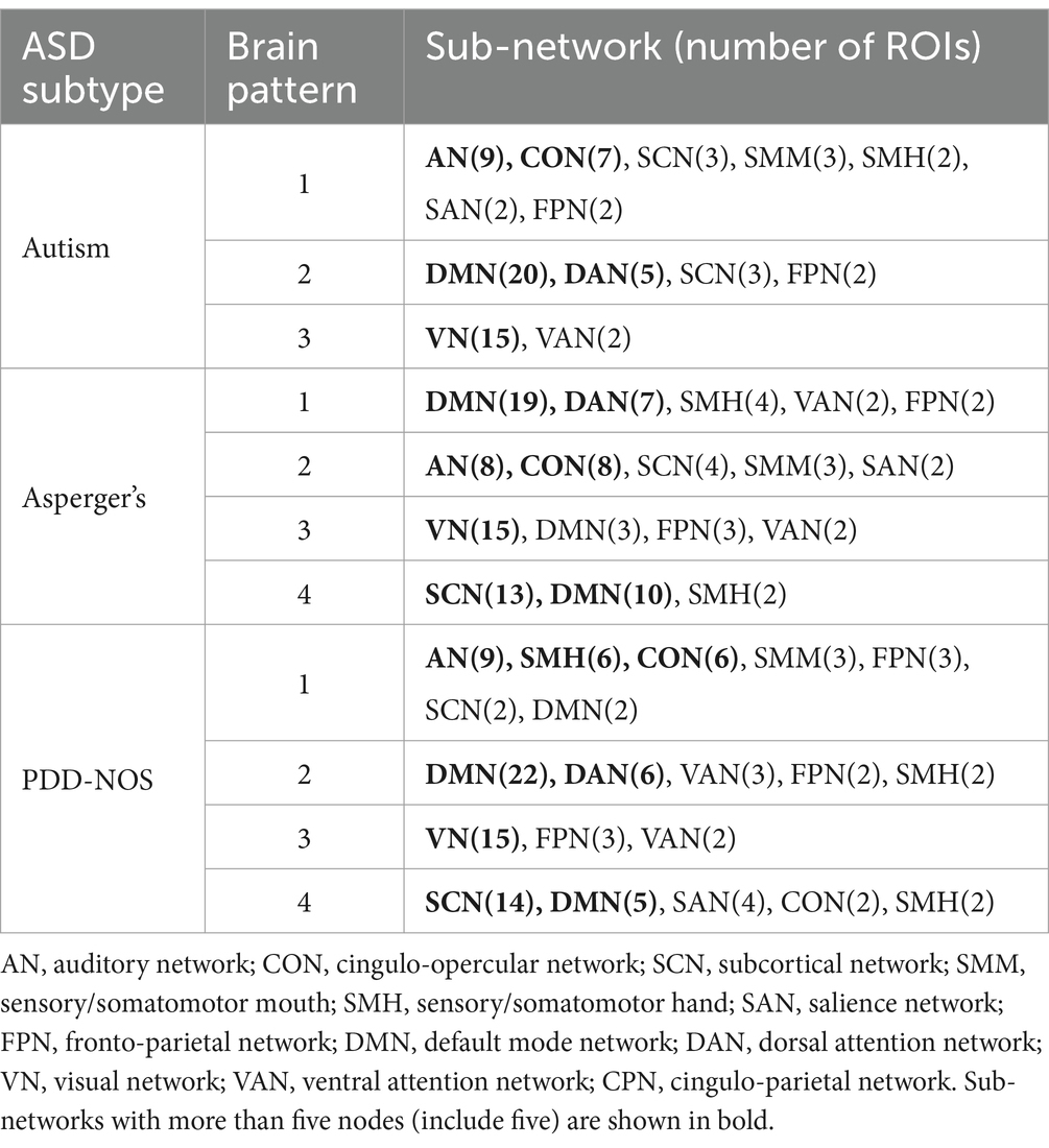
Table 3. Sub-networks involved in brain patterns.

3.2 Inter-comparison of the ASD subtypes

Figures 3–5 show the results of the inter-comparison of the ASD subtypes for ALFF, fALFF, and GMV, respectively. In terms of ALFF, as shown in Figure 3, the number of different ROIs between autism and Asperger’s was much greater than that in the other two conditions, with 27 significant nodes. However, there was no ROI shown in the comparison of PDD-NOS and Asperger’s, indicating that the difference between PDD-NOS and Asperger’s in ALFF was not significant at the level of 0.05. The differences between autism and Asperger’s are mainly focused on the ROIs from the DMN, SCN, VN, and some scattered ROIs from the SAN, CON, DAN, CPN, VAN, and FPN (only one ROI for each). The ROIs with significantly higher ALFF values were mainly in the frontal and temporal lobes, whereas the ROIs with significantly lower ALFF values were mainly in the parietal and occipital lobes. The significant ROIs in the autism vs. PDD-NOS comparison are much fewer, with only four nodes from DMN and FPN, which are mainly focused on the frontal lobe and insula cortex.

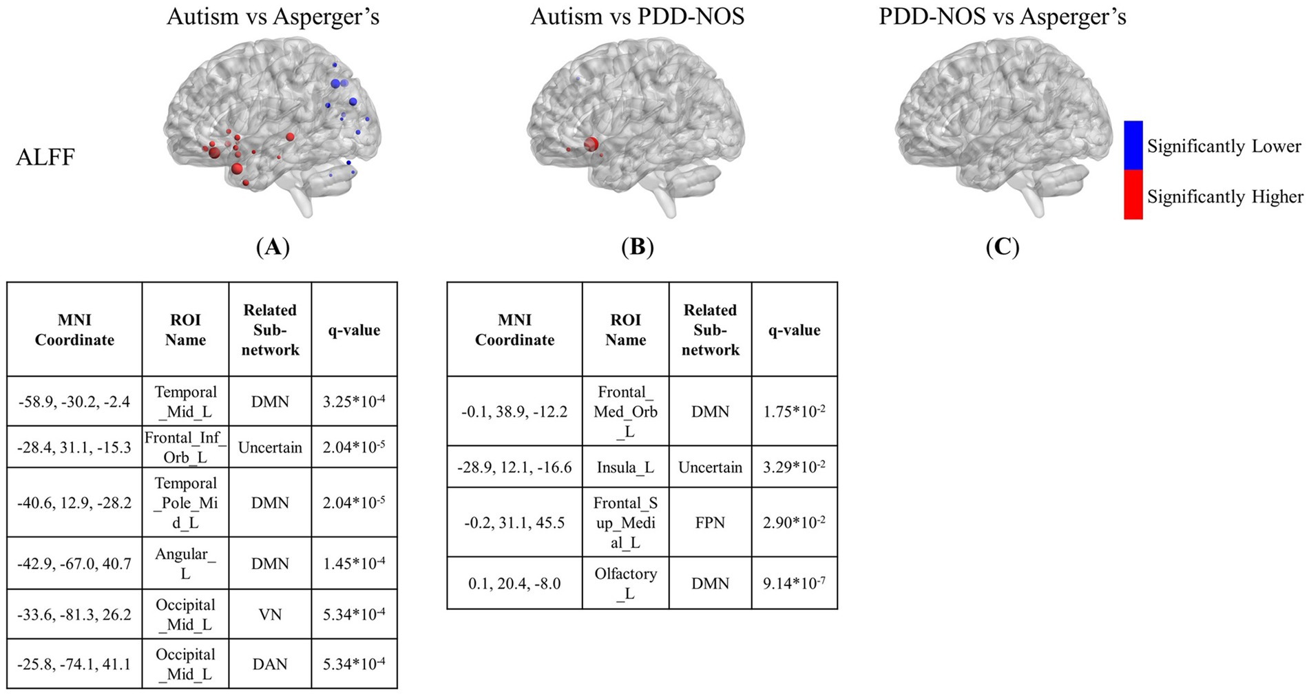
Figure 3. The results of the inter-comparison for ALFF: (A) is the result of the comparison between autism and Asperger’s; (B) is the result of the comparison between autism and PDD-NOS; (C) is the result of the comparison between PDD-NOS and Asperger’s. The tables under each subgraph show the ROIs with the top five of the smallest q-values (if there are not enough ROIs, then all surviving ROIs are shown). It should be noted that the q-values in this study are p-values after FDR correction. The sizes of the ROIs in the figure are related to their q-values. A larger ROI node indicated a smaller q-value, showing greater significance in the t-test. AN, auditory network; CON, cingulo-opercular network; SCN, subcortical network; SMM, sensory/somatomotor mouth; SMH, sensory/somatomotor hand; SAN, salience network; FPN, fronto-parietal network; DMN, default mode network; DAN, dorsal attention network; VN, visual network; VAN, ventral attention network; CPN, cingulo-parietal network.

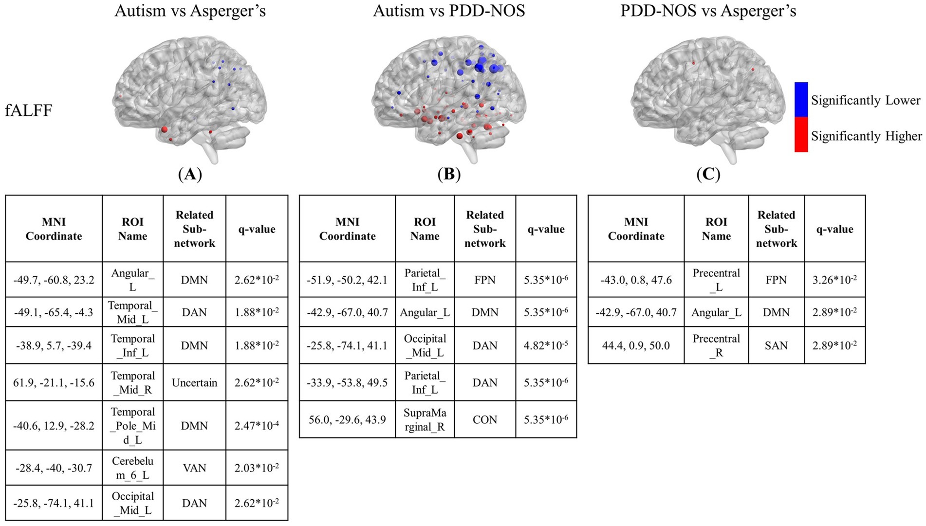
Figure 4. The results of the inter-comparison for fALFF: (A) is the result of the comparison between autism and Asperger’s; (B) is the result of the comparison between autism and PDD-NOS; (C) is the result of the comparison between PDD-NOS and Asperger’s. The tables under each subgraph show the ROIs with the top five smallest q-values. AN, auditory network; CON, cingulo-opercular network; SCN, subcortical network; SMM, sensory/somatomotor mouth; SMH, sensory/somatomotor hand; SAN, salience network; FPN, fronto-parietal network; DMN, default mode network; DAN, dorsal attention network; VN, visual network; VAN, ventral attention network; CPN, cingulo-parietal network.

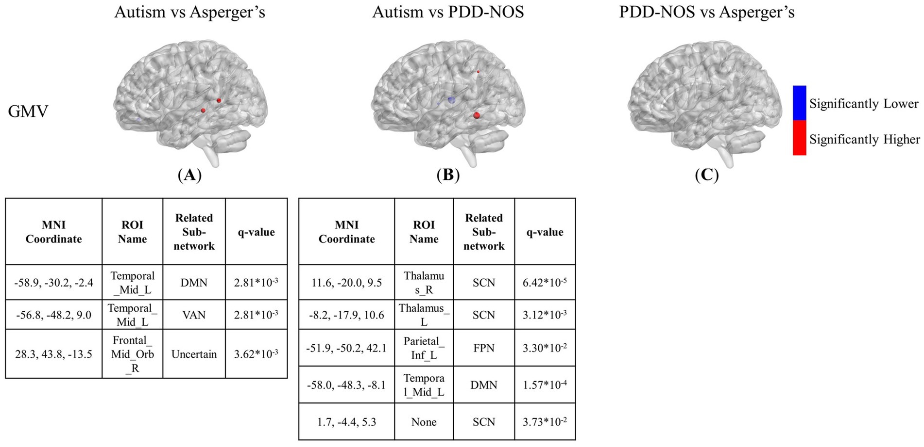
Figure 5. The results of the inter-comparison for GMV: (A) is the result of the comparison between autism and Asperger’s; (B) is the result of the comparison between autism and PDD-NOS; (C) is the result of the comparison between PDD-NOS and Asperger’s. The tables under each subgraph show the ROIs with top 5 of the smallest q-value. AN, auditory network; CON, cingulo-opercular network; SCN, subcortical network; SMM, sensory/somatomotor mouth; SMH, sensory/somatomotor hand; SAN, salience network; FPN, fronto-parietal network; DMN, default mode network; DAN, dorsal attention network; VN, visual network; VAN, ventral attention network; CPN, cingulo-parietal network.

In terms of fALFF, the situation is the opposite to that of ALFF. The differences between autism and Asperger’s in the fALFF are not as many as in the ALFF. As shown in Figure 4A, the significantly different ROIs were mainly focused on the DMN, DAN, VAN, and FPN, with scattered ROIs from the SCN and CON. The DMN still showed the most different ROIs in the comparison, while ROIs from the DAN and FPN of the autism group showed significantly lower fALFF values than those of the Asperger’s group. The comparison between autism and PDD-NOS showed significantly more significant nodes than the other two conditions, with 86 ROIs appearing to be significantly different between the two subtypes. Unlike the condition of autism vs. Asperger’s, the SCN from the autism group showed the most different nodes compared with the PDD-NOS group, where 19 ROIs showed significantly higher fALFF values. Nodes from the DMN, DAN, VAN, and FPN also appear in the comparison. In addition, nodes from VN and CON show differences that are not found in the comparison between autism and Asperger’s condition. There were only three nodes showing differences between Asperger’s and PDD-NOS, with two of them from the precentral gyrus and one from the angular gyrus.