1 Introduction

Evolution endowed neural systems with a level of complexity that is infeasible to emulate in silico without trade-offs. For instance, human brains contain 86 billion neurons, with a substantial metabolic cost of about 20% of the total body energy budget (Herculano-Houzel, 2012). In addition to that, many synaptic connections between neurons, which are a crucial part of neuroscience research, are not static; they are rather plastic entities that change according to activity, thereby altering the dynamics of the associated networks (Feldman, 2012). Aside from the sheer scale and dynamic nature of neural architecture, neurons operate continuously, processing and transmitting information in real time. Considering these complexities, alongside myriad other sources of intricacy within neural systems, it is unsurprising that simulating even a small, simplified subset of these networks on modern computers can become impractical, primarily due to the substantial memory requirements involved.

One of the central complexities we addressed in this work revolves around synaptic plasticity. Within this context, Spike-Timing-Dependent-Plasticity (STDP) holds a prominent position. STDP represents a simple yet powerful plasticity rule that reproduces numerous experimental findings in neurobiology (Bi and Poo, 1998; Markram et al., 2011). Nevertheless, its computational demands can present challenges when translated into the digital realm.

To illustrate this, consider a network comprising N neurons. In this scenario, an N×N crossbar structure is often employed to store connectivity variables, such as synaptic weights. When a neuron emits a spike, both outgoing and incoming connections may necessitate updates, contingent upon the spiking activities of post- and presynaptic neurons, respectively. Handling plasticity operations related to outgoing connections is straightforward since conventional memory arrays support parallel row-wise access (Seo et al., 2011; Knight and Nowotny, 2018). In contrast, the column-wise access (or “reverse” access, as opposed to “forward” access) linked with incoming synapses is inefficient, frequently relying on additional operations to pinpoint the connected presynaptic neurons (Alevi et al., 2022) or allocating separate data structures dedicated to these connections (Knight and Nowotny, 2018). These processes, however, contribute to increased computation time and expanded memory footprint (Pedroni et al., 2019).

Alternative crossbar architectures can be used to address these inefficiencies in column-wise access, thereby promoting scalability and on-chip learning (Seo et al., 2011; Frenkel et al., 2018). Nonetheless, using a synapse crossbar has a drawback: nonexistent connections within the network still occupy physical space. This compromises silicon area and is particularly problematic for sparse, recurrent networks (Pedroni et al., 2019). Instead of implementing synapse crossbars or introducing dependencies on additional state variables, alternative approaches focus on delaying weight updates. For example, in neuromorphic boards such as SpiNNaker, presynaptic spikes trigger acausal weight updates as usual, but causal updates due to postsynaptic spikes occur only when another presynaptic spike is delivered at the corresponding synapse (Diehl and Cook, 2014, but see Bogdan et al. (2020), for a more current implementation). With Loihi, Davies et al. (2018) defined a learning epoch time, after which plasticity takes place. Pedroni et al. (2019) pursued a similar approach and demonstrated that pointer-based data structures, such as compressed sparse row, serve as efficient alternatives for memory storage. More importantly, as previously shown, the inefficiencies associated with reverse access required by postsynaptic spikes can be circumvented by slightly delaying weight updates. In other words, both causal and acausal updates can be executed with forward access driven by presynaptic custom events, provided that spike time information is adequately stored. This strategy facilitates contiguous memory allocation, which leads to improved memory access and faster simulation of Spiking Neural Networks (SNNs; Bautembach et al., 2021). In essence, more efficient methods of accessing memory in digital systems have enabled a wealth of scalable and fast simulation platforms (Thakur et al., 2018; Frenkel et al., 2023).

Research in computational neuroscience deals with highly complex systems, so simulation strategies are not limited to improving memory access efficiency. Simplifications are often adopted to create tractable models that can be integrated into large network models (Teeter et al., 2018; Chen et al., 2022; Pagkalos et al., 2023). Importantly, simpler models can be exploited to optimize a design. For instance, a shared update logic (e.g., exponential decay) allows a time-multiplexing scheme, which leads to better resource utilization and scalability (Wang and van Schaik, 2018; Modaresi et al., 2023).

In this work, we delve into an innovative alternative to STDP for digital hardware that enhances efficiency and scalability and reduces memory footprint. We achieved this by enforcing contiguous memory allocation and a reduced model complexity. Specifically, we have devised a custom event mechanism that facilitates weight updates (causal and acausal) with forward access only. Since we were interested in the sparsity of more realistic neuronal connectivity, we tackled a pointer-based structure for weight storage. Furthermore, our investigation demonstrates the feasibility of reducing the number of state variables used per neuron for computing plastic changes, thus further increasing scalability. Finally, we considered the implications of this reduction on the network statistics.

2 Materials and methods 2.1 State variables

The simulations described here were carried out using Brian2 (Stimberg et al., 2019) with its graphics processing unit backend (Alevi et al., 2022). The equations governing the membrane potential (Vm) and postsynaptic potential (PSP) are

Vm[t+1]=αmVm[t]+αmdtPSP[t]τm    (1)

and

PSP[t+1]=αsynPSP[t],    (2)

respectively, where τm = 20 ms and τsyn = 5 ms. We adopted αm = τm/(τm+dt), αsyn = τsyn/(τsyn+dt), and dt = 1 ms. Equations 1, 2 represent simple dynamics of LIF neuron models and current-based synapses. A spike is generated if the Vm>Vthr = 20 mV, in which case Vm is set to Vreset = 0 mV and the cell becomes refractory for 2 ms. A crucial distinction herein is that the “ownership” of state variables was engineered to minimize memory footprint. Specifically, instead of allocating one PSP for each synaptic connection, our model assigns one for each neuron.

A presynaptic spike from an excitatory (inhibitory) neuron i connected to a neuron j increments (decrements) the PSP value according to the synaptic weight wji. Regarding synaptic plasticity, changes in the strength of excitatory-excitatory connections wji are regulated by the interaction between spikes and their timing information. This information is stored in traces. Similarly to other state variables, each neuron holds one trace x(t), which is increased by Δx whenever this neuron emits an action potential. The evolution of x over time can be defined as

x[t+1]=αxx[t],    (3)

where αx = τx/(τx+dt).

2.2 Plasticity implementation

In conventional STDP, wji can be updated as

wji={wji−ηxj                    (4)wji+ηxi,                              (5)

with a learning rate η and state variable x as defined in Equation 3. Equation 4 is computed upon the occurrence of a presynaptic spike, while Equation 5 is evaluated whenever there is a postsynaptic spike. In other words, spikes must be detected and stored in memory. The state variables associated with those spiking neurons must then be fetched from memory so that acausal or causal updates can occur.

During our study, we signaled a spike by momentarily setting the most significant bit of a neuronal x trace to 1. This was accomplished in Brian2 by simply setting the trace to a negative value, but the positive sign had to be restored by the end of the simulation time step. Since we wanted to avoid the overhead of reverse memory access triggered by a postsynaptic spike, we explored a methodology that allows for weight updates exclusively through forward access. Essentially, whenever a presynaptic neuron was active (see definition below), all the postsynaptic traces were retrieved from memory. A negative presynaptic trace paired with a positive postsynaptic trace triggered acausal updates, whereas the opposite caused a causal update. No updates were performed when both neurons fired simultaneously.

In our simulations, we have defined a neuron as active when its x variable exceeds a certain threshold xthr. When a neuron spikes, the outgoing weights are tentatively updated, that is, weights change only under the right conditions. This process is repeated in subsequent time steps as long as the presynaptic trace remains above the designated threshold. If a postsynaptic spike eventually occurs, a causal update can take place. Notably, there is no necessity for reverse access to locate the presynaptic neurons; all active neurons are already triggering the necessary updates based on the temporal information carried by the traces.

Our scheme can be summarized as follows: As long as a neuron is active, outgoing weights are updated according to

wji={wji-ηxjif xi<0∧xj>0wji+ηxi,if xi>0∧xj<0    (6)

where ∧ is a simple AND logic operator. Note that we can cast the above equations as a conventional STDP rule if the first condition is “neuron i spiked” and the second is “neuron j spiked.”

Figure 1 presents a visual illustration. No weight updates are performed when a single neuron is active, but memory fetches of postsynaptic variables are carried out to detect upcoming events (Figures 1A, B). When another neuron becomes active (Figure 1C), a causal update is detected and fulfilled. Note that no reverse memory accesses were necessary. No updates are required in Figure 1D, but memory fetches continue.

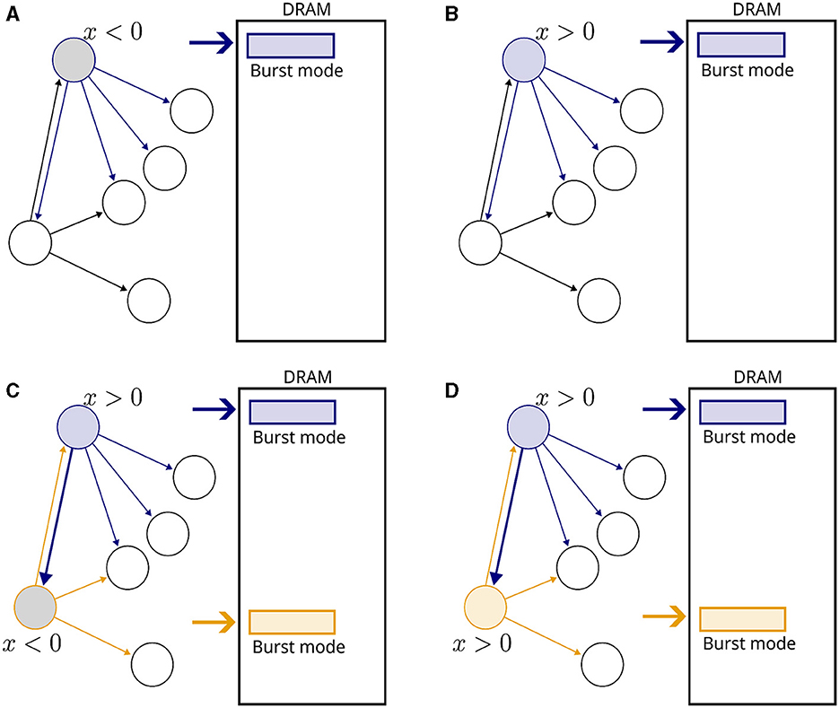
Figure 1. Illustration of the proposed plasticity scheme. Neurons are represented by circles and connections by arrows. Inactive neurons are displayed in black without filling. A rectangle represents a DRAM memory cell. (A) A neuron becomes active, indicated by a blue outline. The gray filling means that x < 0. All fan-out variables are fetched from the DRAM in burst mode. (B) In the next time step, x becomes positive and fetching from memory continues. (C) Another neuron becomes active, indicated by a orange outline. The connection from blue to orange neurons is potentiated, and new memory fetches are triggered. (D) In the subsequent time step, no weight updates take place because both neurons are inactive, but memory fetches continue.

To emulate our simulation pipeline with Brian2, we created a custom event to capture when a neuron was active. This enabled synaptic objects access to state variables and perform the required operations. The general scheme is summarized in Figure 2, where each block on the left column represents the order, from top to bottom, in which Brian2's execution slots were scheduled in a single time step. The calculations assigned to each block are shown in the middle column. Additionally, in the right column, we indicated how this pipeline could be incorporated into an advanced time-multiplexing approach, which splits slots into time-driven and event-driven modules (Wang and van Schaik, 2018).

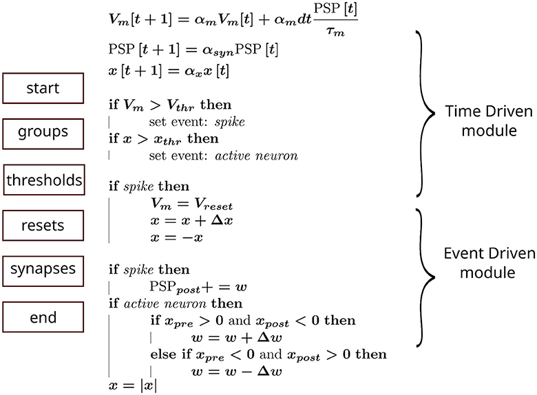
Figure 2. Hardware emulation using Brian2. Each block on the left represents the computation groups available in Brian2. They were scheduled in this sequence (from top to bottom) to approximate hardware behavior. The equations in the middle show the operations performed in each block, whereas the curly braces on the right indicate the corresponding hardware module emulated.

2.3 Simulations performed

To test our approach, we initially simulated simple scenarios in which an input layer of neurons projected onto postsynaptic neurons in a feedforward manner. In these experiments, presynaptic spikes were either generated deterministically or stochastically. The primary objective was to replicate expected outcomes, such as dependence of synaptic modifications on spike timing (Bi and Poo, 1998) and a bimodal distribution of weights (Song et al., 2000). Unless otherwise specified, the parameters related to plasticity were set to the values shown in Table 1.

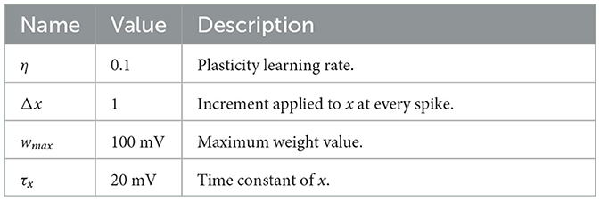
Table 1. Parameters and descriptions of plasticity model.

Conventional models of how a synapse strength is modified through STDP typically incorporate traces for both potentiation and depression. By doing this, it is possible to tune parameters so that synaptic weakening is larger than strengthening, which leads to desirable properties (Song et al., 2000). Our models, however, possess a single trace per neuron, so we relied on other strategies. As heterogeneity is associated with improved stability and robustness (Perez-Nieves et al., 2021), we sampled each τx from a uniform distribution in some of our simulations.

We also investigated and compared the number of memory accesses required for different strategies. While various factors influence memory access in an actual digital system, like latency, locality principle, burst mode, and bandwidth, we simplified the scenario by assuming that accessing a single memory position had a generic cost of 1. This interpretation helps understand the cost of performing STDP in a digital system, especially since reading a single state variable may add many clock cycles of overhead (Pedroni et al., 2019). Clearly, the chosen data structure impacts the access pattern. Therefore, we considered a pointer-based storage structure due to its small memory footprint in sparse, recurrent networks.

The storage cost of the proposed models can be separated into two parts—neurons and synapses. The cost for neurons is calculated as NvarNbitsNt, where Nvar represents the number of state variables (Nvar = 3), Nbits is the bit resolution (Nbits = 64), and Nt is the total number of neurons. On the other hand, the cost for synapses can be calculated as NpreρNpostNbits+NpreρNpostlog2Npost+Nprelog2(NpreρNpost), where ρ is the connection probability. The first term represents the bit resolution of synaptic weights for each connection in the weight table, while the second term depicts the address of the postsynaptic neuron within that table. The last term pertains to the pointer table, which maintains the outgoing connections for each presynaptic neuron.

The computations performed during time-driven and event-driven modules are different, and so is the access cost of each. During the time-driven module, neuronal state variables are loaded, resulting in a cost of 3Nt. For the event-driven module, forward access incurs a cost of Nprea(2+ρNpost), where Nprea is the number of active presynaptic neurons associated with plastic weights (i.e., those whose axons make synaptic connections with other excitatory neurons). Considering that reverse access is achieved by using forward access to traverse weight tables to find the connected neuron pairs, the cost can be expressed as Nposta(Npre+NpreρNpost). Note that accesses depend on the number of active neurons at every time step, so the size and rate of the neuronal population directly impact these metrics. Moreover, although using fewer state variables per neuron can already decrease storage requirements and memory access overhead, our study concentrated on the memory access complexities related to STDP during the event-driven module.

In our investigation, we compared the access costs associated with our forward-only access strategy and a conventional approach that also includes reverse access triggered by postsynaptic spikes. For the sake of simplification, the computational overhead of fetching the start and end addresses of the weight table was not incorporated into the analysis, as it should be small compared to the weight table itself.

Since we aim to improve the scalability of SNNs endowed with plasticity in digital hardware, we also tested our approach on a large-scale simulation of a balanced network (Morrison et al., 2007), illustrated in Figure 3. The network comprised 90,000 excitatory neurons and 22,500 inhibitory neurons, with a connection probability of 0.1 (represented by the symbol ρ). The number of connections per neuron was about 104, and the total number of synapses in the network was in the order of 109. Neurons were driven by spike trains generated from 9,000 independent Poisson processes at 2.32 Hz.

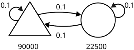
Figure 3. Schematic of the balanced random network model. The triangle represents the excitatory neurons, and the circle represents the inhibitory neurons. The number of neurons in each population is written under the corresponding symbol. Arrows indicate connections between populations, each with a specific probability.

The plasticity rule in Equation 6 was slightly modified to

wji={wji-ηαwjixjif xi<0∧xj>0wji+ηw01-μwjiμxiif xi>0∧xj<0    (7)

and applied to excitatory-excitatory connections. The additional parameters for the simulation are shown in Table 2. Note that a neuron was not allowed to connect to itself and that there were no instantaneous spike propagations.

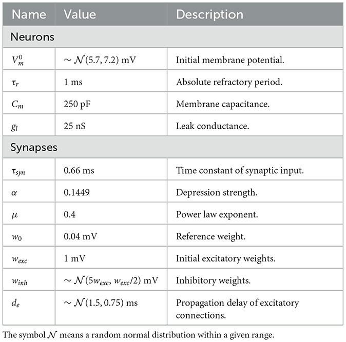
Table 2. Parameters and description of balanced network with STDP.

Morrison et al. (2007) implemented their synaptic currents as an α function, which is more complex than the model we adopted. To obtain PSPs similar to their work, we utilized wexc = 25pA/gl = 1mV. Moreover, PSPs peaked around 0.14 mV, with a rise time of 1.7 ms and a half-width of 8.5 ms.

3 Results 3.1 Simple STDP benchmarks

We began by examining a simple scenario where a single synapse underwent multiple potentiations and depressions. Figure 4A illustrates the strength of a synaptic weight over time when multiple STDP protocols (indicated by Roman numerals) were applied. The original and proposed implementations yielded similar values, although minor errors were accumulated over time.

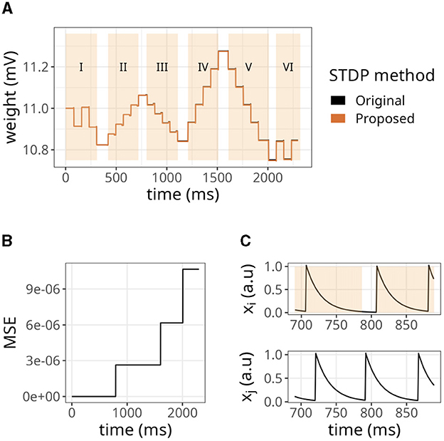
Figure 4. Evolution of state variables in time with the STDP implementation proposed. (A) Weight changes of the proposed and original STDP implementations during multiple protocols, namely random (I), weak potentiation (II), weak depression (III), strong potentiation (IV), strong depression (V), and random again (VI). On each protocol, a pair of pre- and postsynaptic neurons were forced to spike in a desired order to elicit the observed updates. (B) Mean squared error (MSE) between the original and proposed traces shown in A. The traces in A are very close to one another, so the MSE is used to highlight the small differences between them. (C) Traces from pre- (xi) and postsynaptic (xj) neurons, where orange overlay shows regions where the presynaptic neuron was active.

As shown in Figure 4B, the mean squared error (MSE) between them was minimal but increased in the same interval. The difference between our approach and the original formulation lies in the precision of traces. In the original formulation, even if the trace value is minimal, it still causes a slight increase or decrease in the synaptic weight. In contrast, we set a threshold of xthr = 0.02 in our approach, which means that traces below this value were considered insignificant and the presynaptic neuron was considered inactive. Hence, no weight updates were performed. Figure 4C shows that our approach introduced an error around 791 ms where xi<xthr. As a result, the postsynaptic spike did not trigger any changes in the synaptic weight. Accordingly, a threshold of xthr = 0, would introduce no errors (not shown).

To further evaluate the STDP proposed, we replicated some established properties of this plasticity rule. Figure 5A shows the dependence of synaptic modification on spike timing. For the experiment, we connected each pair of neurons with an initial weight value of 50 mV, and a fixed spike timing between them was repeated 100 times. The results were similar to the original formulation. Nevertheless, as shown above, minor errors accumulated (see Figure 5B).

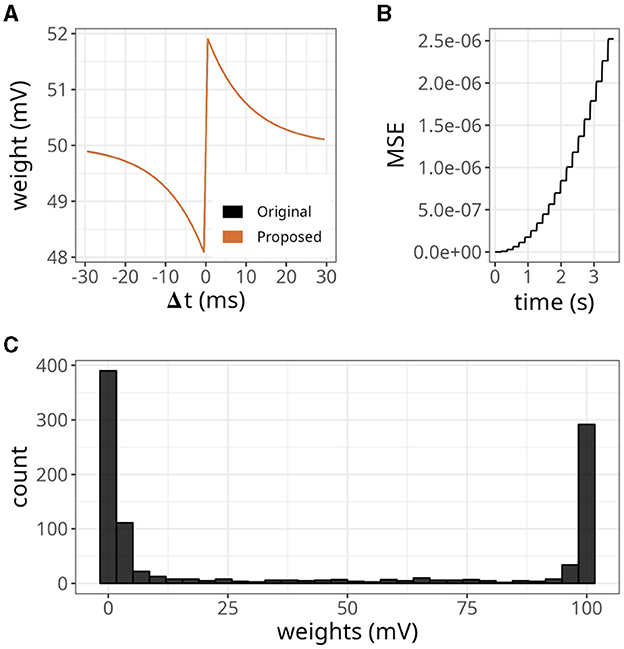
Figure 5. Distribution of weights after undergoing plasticity under the proposed STDP implementation. (A) Weight values as a function of the difference between pre- and postsynaptic spikes —Δt = tpost −tpre. Both original and proposed implementations are shown. (B) Mean squared error (MSE) between the original and proposed traces shown in (A). (C) Bimodal distribution of weights under the proposed STDP implementation.

In our STDP implementation, the distribution of plastic synaptic weights in a network with 1000 presynaptic neurons firing at 15 Hz and one postsynaptic neuron converged to a bimodal distribution. This is illustrated in Figure 5C. Most of the weights were either close to zero mV or close to the maximum value of wmax = 100 mV. It is worth noting that the selected values of τx played a significant role in shaping the distribution profile. The range of τx values used in the above results varied between 5 and 15 ms and were randomly sampled from a uniform distribution. The initial weights were drawn from a gamma distribution with k = 1 and θ = 17.5. However, the initial weight values did not significantly impact the outcome as long as the postsynaptic neuron was firing.

3.2 Efficiency measurements

In the previous simulations, we observed that reducing the value of xthr led to fewer deviations from the original STDP formulation. However, it also increased the number of memory accesses performed at every time step. To further understand the impacts of different threshold values, we calculated the number of memory accesses required for the bimodal distribution benchmark, which highlights some desirable properties of STDP. Additionally, we set the value of wmax to 0.4 to limit the final firing rate of the postsynaptic neuron. Since τx can affect the distribution of weights, we adjusted its interval to be between 16 and 26 to ensure a bimodal distribution.

The results are displayed in Figure 6. Our approach, with various xthr, was compared to a conventional formulation (i.e., forward and reverse access) labeled as “control.” At the start of the simulation, the number of spikes emitted by the postsynaptic neuron reached values close to 40 but gradually decreased over time (Figure 6A). This is a relevant observation because when the postsynaptic neuron is not spiking, the number of memory accesses is determined by all active presynaptic neurons driving forward accesses.

Figure 6. Analysis of the number of memory access (mems) over time. (A) Histogram of spike counts of the postsynaptic neuron over time. (B) Number of memory accesses at each time step for different implementation strategies. The time interval considered ranged from 0 to 100 ms on the left panel, and from 99.5 to 100 s on the right panel. (C) Boxplots of memory fetches for each time step. Individual data points are also shown on top of the boxes. The time interval considered ranged from 0 to 250 ms (left panel), and from 99.5 to 99.75 s (right panel).

Since we connected all 1,000 presynaptic neurons firing at 15 Hz to a single postsynaptic neuron, the control case shown in Figure 6B displayed around 15 memory accesses at most time steps. However, postsynaptic spikes caused peaks that reached values slightly above 1,000 due to reverse access. In contrast, our approach was not affected by postsynaptic spikes, but it yielded numbers of memory accesses higher than the control case. When we set xthr = 0, neurons could not become inactive (i.e., x = xthr) due to the high precision of double-precision floating-point numbers. Therefore, the number of memory accesses in this case increased persistently until the maximum, which was 1,000. As we increased xthr (e.g., to 0.02 or 0.1), more neurons became inactive, causing the number to converge to a smaller value at the end of the simulation (see right panel of Figure 6B).

In Figure 6C, we show the boxplots of memory fetches for each time step over 250 ms at the start and end of the simulation. From the data, it appears that the effects of reverse access are not significant in the control case. However, it is worth noting that the previous simulations only involved low spiking rates and a single postsynaptic neuron.

Figure 7 demonstrates a scenario with a higher number of postsynaptic neurons and slightly higher firing rates, around 25 Hz. The data points were taken from a time interval of 250 ms after both traces converged to a stable value. Upon closer inspection, it becomes apparent that our approach was not affected by the increase in postsynaptic neurons (indicated at the top of each panel). On the other hand, for the control case, not only did the maximum value increase significantly as the number of postsynaptic neurons increased, but also the average. In fact, with 100 postsynaptic neurons, the average value of the control case was higher than the proposed approach.

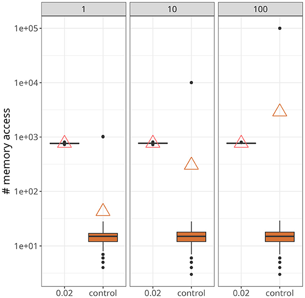
Figure 7. Statistics of memory accesses. Each boxplot was calculated based on ten simulation runs. Triangles denote the average memory access in each case. The number at the top of each panel represents the number of postsynaptic neurons. In all panes, our approach, with xthr = 0.02, was compared with the conventional (i.e., control) formulation.

3.3 Large-scale networks

As excitatory weights in a network increase due to STDP updates, the stability of the system can be compromised. This can be particularly problematic in large networks, where each neuron makes thousands of connections. In Figure 8A, we have shown the final weight distribution (i.e., after 200 s) of a large-scale network endowed with the plasticity rule of Equation 7. To facilitate comparisons with the original model (Morrison et al., 2007), we multiplied our weights by gl to get values in pA. Although the initial value of those weights was 25 pA, they evolved to form an unimodal distribution. The final shape was similar to a normal distribution with a mean of 25 and a standard deviation of 2. Note that the maximum synaptic strength in these experiments was set to wmax = 1, 000 mV, which indicates that the weights settled to a stable value without saturation.

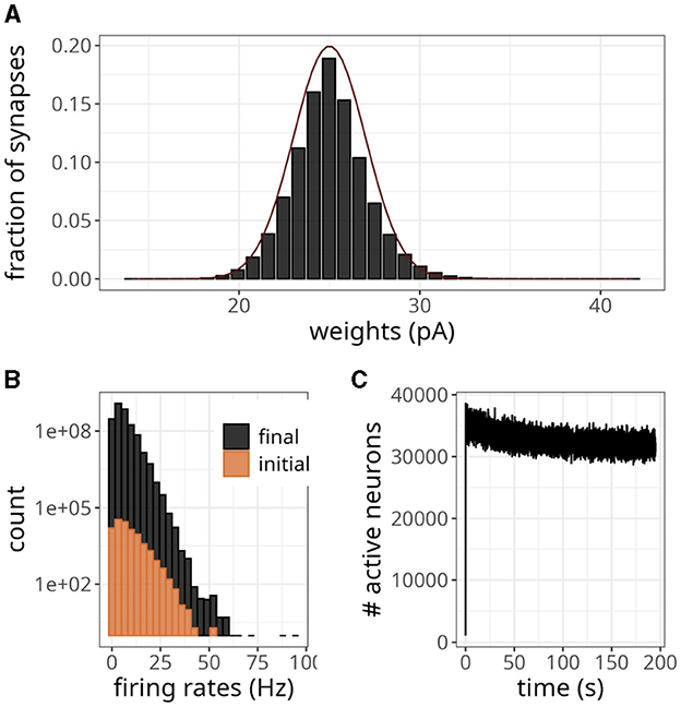
Figure 8. Large-scale balanced network with plasticity. (A) Histogram of synaptic weights. The dark line represents a Gaussian distribution with a mean of 25 and a standard deviation of 2. (B) Distribution of firing rates across neurons in the initial and final 2 s. (C) Number of active neurons over time for plasticity updates.

The statistics of the network were akin to an asynchronous and irregular regime, with a mean firing rate of 5.70 Hz and CV of 0.90. The spike variability was high, as indicated by a Fano factor of 5.11. The histogram in Figure 8B shows that only a few neurons exhibited high firing rates, even though the weights were small. The difference in count values suggests that regular activity of the network at the beginning of the simulation produced an intense blanket of inhibition, effectively silencing some neurons. As irregularity increased, other neurons became more susceptible to excitatory drive, yet the average number of active neurons revealed a decreasing trend (Figure 8C).

According to the magnitude of the network analyzed, the storage cost associated with neurons and synapses is around 2.7 MB and 12.78 GB, respectively. Figure 8C illustrates the pattern of active neurons over time, which shows an initial peak followed by a steady decrease. This number fluctuated around a mean of ~32,000 per time step, probably as a result of the high activity levels of some neurons (see Figure 8B). Nevertheless, this number is lower than the worst-case scenario of 90,000.

As pointed out by the authors who first proposed Equation 7, if the parameter α was slightly smaller than αp=w*w0μ-1, where w* is the fixed point of the synaptic weight distribution, depression would not be able to counteract strong potentiations induced by fast oscillations effectively. To test this scenario in our model, we decreased α by 2%, going from α = αp = 0.1449 to α = 0.1420. Figure 9 shows the resulting weight distribution after 13 s of simulation. Most weights were still concentrated around the mean of 25 pA, but a small proportion of synapses were further strengthened, with weights extending up to 82 pA. Despite the emergence of some denser regions suggesting clustering, these highly potentiated synapses were predominantly dispersed and lacked a discernible pattern. Simulating for 20 s resulted in even stronger weights, with a small fraction sparsely distributed between 60 pA and the maximum weight of 25 nA.

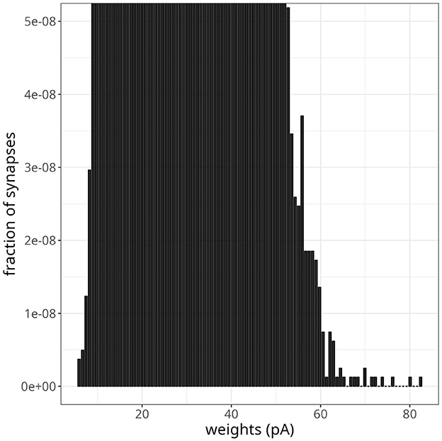
Figure 9. Instability in balanced network with plasticity. Histogram of synaptic weights after a simulation time of 13 s. The plot was zoomed in to visualize higher-weight but less frequent synaptic connections.

We wanted to verify whether our model could replicate a bimodal distribution, so we replaced the previous plasticity rule with Equation 6. Figure 10A shows the resulting bimodal profile. Although intermediary values were not negligible, we observed prominent peaks close to the minimum and maximum values. To generate this distribution, we set the maximum weight to wmax = 0.5 mV and sampled the initial wexc from a random uniform distribution. To sample the inhibitory weights as in Table 2, we selected the reference excitatory weight as wexc = 0.25 mV. We could have adopted a higher cap without compromising this weight distribution, but we wanted to avoid high firing rates.