1 Introduction

Ultrasound (US) is pivotal in the diagnosis, treatment and follow-up of patients in several medical specialities such as cardiology, obstetrics, gynaecology and hepatology. However, the quality of acquired images varies greatly depending on operators’ skills, which can impact diagnostic and interventional outcomes (1).

Providing guidance or automation for the image acquisition process would allow for reproducible imaging, increase both the workflow efficiency and throughput of echo departments and improve access to ultrasound examinations. This requires an intelligent system, capable of acquiring images by taking into consideration the high variability of patient anatomies.

Several works are investigating US acquisition automation but commercially available systems do not go beyond teleoperated ultrasound (2). Recent research towards autonomous navigation has used imitation learning (3) and deep reinforcement learning (4, 5). While these methods achieve varying degrees of success, they struggle to adapt to unseen anatomies, can only manage simple scanning patterns or are tested on small datasets.

The main advantage of a simulation environment is the ability to generate views that occur when operators navigate to a given standard view or anatomical landmark but are not saved in clinical routine. These datasets, which we call navigation data, can also contain imaging artefacts (e.g. shadowing caused by ribs). Hence, recent ultrasound image synthesis methods using neural networks (6, 7) face significant challenges in generating these views due to the necessity of comprehending ultrasound physics and the unavailability of large-scale datasets of complete ultrasound acquisitions. Besides, learning-based approaches for navigation (5) require a large number of images for training, including non-standard views, which are not available in classical ultrasound training datasets.

Using a simulation environment to train such a system would have several benefits. The trained model could learn while being exposed to a varying range of anatomies and image qualities, hence improving its robustness, and the training could be done safely, preventing the wear of mechanical components and potential injuries. This simulation environment should be: (1) Fast, to enable the use of state-of-the-art reinforcement learning algorithms. (2) Reproduce patients’ anatomies with high fidelity. (3) Recreate attenuation artefacts such as shadowing. Moreover, exposing the system to a wide range of anatomies requires large-scale data generation capabilities, meaning the pre-processing of data must be streamlined.

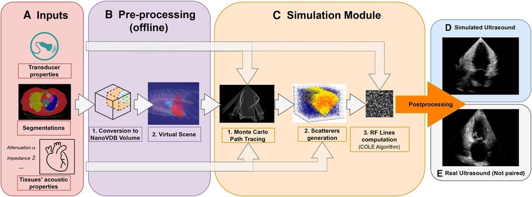
This paper presents an ultrasound simulation pipeline using Graphical Processing Unit (GPU) based ray tracing on NVIDIA OptiX (8), capable of generating US images in less than a second. By combining networks capable of segmenting a wide range of tissues and a volumetric data representation, we overcome the scene modelling limitations of previous mesh-based simulation methods, enabling efficient processing of numerous datasets from different modalities. Our pipeline, described in Figure 1 takes as input segmentations of the organs of interest and, coupled with user-defined transducer and tissue properties, generates a simulated US by combining Monte Carlo path tracing (MCPT) and convolutional approaches.

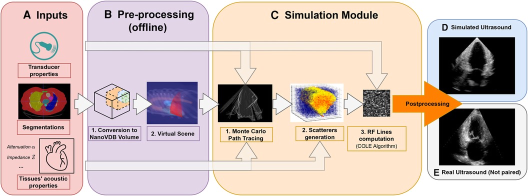
Figure 1. Simulation Pipeline. Using input segmentations from other modalities, transducer and tissue acoustic properties (A), we convert the segmentation to a NanoVDB volume (B.1) for ray tracing on the GPU. (B.2) shows a volume rendering of the ray tracing scene with various organs and the transducer’s fan geometry. We model the sound waves as rays and perform ray tracing to simulate their propagation (C.1). We then generate a scattering volume (C.2) and compute the RF lines (C.3). Time-gain compensation and scan conversion are performed to yield the final simulation (D). A real ultrasound is shown for qualitative comparison (E).

Our contributions are the following:

• Our pipeline is able to generate images from a large number of datasets from other modalities. Using an efficient GPU volumetric representation that allows for the modelling of arbitrary patient anatomies, and a Monte Carlo path tracing algorithm, we are able to synthesize more than 10,000 images per hour using a NVIDIA Quadro K5000 GPU. Furthermore, we demonstrate scalability by generating images from 1,000 CT patient datasets in our experiments. In contrast, existing ray tracing methods limit their experiments to datasets one or two orders of magnitude smaller.

• We extensively validate the ability of our pipeline to preserve anatomical features through a phantom experiment by looking at distances and contrast between structures. Ultrasound image properties are further assessed by looking at first-order speckle statistics.

• We demonstrate the usability of our pipeline in training neural networks for transthoracic echocardiography (TTE) standard view classification, a task critical in ultrasound navigation guidance. The neural networks were initially pre-trained on synthetic images and subsequently fine-tuned using varying amounts of real data. With around half of the real samples, fine-tuned networks reach a performance level comparable to those trained with all the real data. We also report an improved classification performance when using pre-trained networks, particularly for under-represented classes.

This paper is organised in the following way: In Section 2.1, we provide an overview of relevant ultrasound simulation methods and highlight their limitations in terms of suitability as simulation environments. The next subsections in Section 2. detail our simulation implementation. Experimental results using a virtual phantom and a view classification network are shown in Section 3. This is followed by a discussion and a conclusion.

2 Methods 2.1 Related work

Early methods were attempting to simulate the US image formation process by solving the wave equation using various strategies (9–13). While being accurate, these methods take a substantial amount of time to generate images [in the order of several minutes to hours (9–12)], which is not scalable for large-scale training.

The COLE Algorithm developed by Gao et al. (14) is at the core of Convolutional Ray Tracing (CRT) methods. This approach allows for a fast simulation of ultrasound images with speckle noise by convolving a separable Point-Spread Function (PSF) with a scatterer distribution. Methods in (15–17) replace the ray casting by ray tracing and combine it with the COLE algorithm to simulate images on the GPU. These methods follow a similar methodology where the input volumes are segmented and acoustic properties from the literature are assigned to each tissue. Scatterers amplitude are hyperparameters chosen such that the generated ultrasounds look plausible. Ray tracing is used to model large-scale effects at boundaries (reflection and refraction) and attenuation within tissue. Finally, the COLE algorithm is applied to yield the final image. The method developed in Mattausch et al. (17) distinguishes itself by employing Monte-Carlo Path Tracing (MCPT) to approximate the ray intensity at given points by taking into account contributions from multiple directions.

CRT methods enable fast simulations and the recreation of imaging artefacts. Methods in (15, 17) both make use of meshes to represent the boundaries between organs. However, using meshes comes with a set of issues as specific pre-processing and algorithms are needed to manage overlapping boundaries. This can lead to the erroneous rendering of tissues, hence limiting the type of scene that can be modelled, as reported in Mattausch et al. (17). A further limitation of CRT methods lies in tissue parameterization, where scatterers belonging to the same tissue have similar properties, preventing the modelling of fine-tissue variations, and thus limiting the realism of the images.

Another line of work generates synthetic ultrasound images by directly sampling scatterers’ intensities from template ultrasound images and using electromechanical models to apply cardiac motion (18, 19). These are different from our line of work as they require pre-existing ultrasound recordings for a given patient, while we generate synthetic images from other modalities, which also enables us to simulate different types of organs other than the heart.

Finally, as deep learning has become increasingly popular, the field shifted towards the use of generative adversarial networks (GAN) or diffusion models for image synthesis. These generative models have been used in several ways for image simulation: Either for generating images directly from segmentations (6, 7, 20), calibrated coordinates (21), or for improving the quality of images generated from CRT simulators (22–24). However, using GANs comes with several challenges: For instance, authors in Hu et al. (21) report mode collapse when generating images for poses where training data was not available and authors in Gilbert et al. (6) report hallucination of structures if anatomical structures are not equally represented in datasets. This suggests generative neural networks would struggle in generating out-of-distribution views or with image artefacts such as shadowing. This would be problematic for ultrasound navigation guidance as out-of-distribution views are frequently encountered before reaching a desired standard view.

Methods taking as input low-quality images from CRT simulators seem the most promising, but several works report issues in preventing the GANs from distorting the anatomy (24) or introducing unrealistic image artefacts (22). While CRT methods are limited in realism, they match our requirements (speed, artefacts recreation, anatomical fidelity through accurate geometry) to train navigation/guidance algorithms.

2.2 Pre-processing pipeline

This section presents our novel pre-processing pipeline, shown in Figure 1, which enables large-scale data generation by avoiding technical pitfalls caused by the use of meshes (17), thus allowing us to model any anatomy. Besides, the use of segmentations is essential to implement constraints on the environment for navigation tasks.

Input volumes (Figure 1A) are segmentations obtained from either CT or Magnetic Resonance Imaging (MRI) datasets, which are processed by a four chamber (25) and multi-organ segmentation algorithm (26). The segmentation output contains all the structures relevant for echocardiography, e.g. individual ribs, sternum, heart chambers, aorta, and lungs.

During ray tracing, voxels need to be accessed at random. The access speed is highly dependent on the memory layout of the data. This problem has been addressed by OpenVDB (27) with its optimized B+ tree data structure and by its compacted, read-only and GPU-compatible version, NanoVDB (28). Data in Open/NanoVDB are stored in grids. These grids can be written together into a single file, which we call an Open/NanoVDB volume. We convert the segmentation volumes into NanoVDB volumes (Figure 1B) as described below.

A detailed overview of the pre-processing pipeline is shown in Figure 2. Firstly, the segmentation volume with all labels is converted to a NanoVDB grid (Figure 2iii-1). This grid is used during ray tracing to access a label associated with a given voxel. Then, for each label in the segmentation volume, a narrow-band signed distance function (SDF) is computed such that the distance from voxels in the neighbourhood of the organ to its boundary is known (Figure 2ii). Blue (resp. red) bands represent the voxels with negative (resp. positive) distance to that boundary, i.e. inside (resp. outside) it. The SDF grids are written to the output volume (Figure 2iii-3) and are later used during traversal to compute smooth surface normals by looking at the SDF’s gradient (Figure 2v).

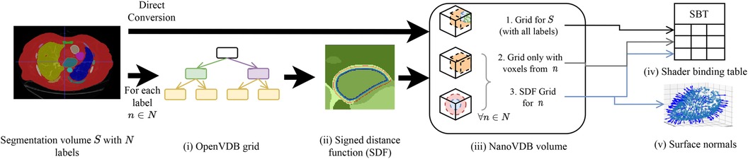
Figure 2. Overview of the pre-processing pipeline. A segmentation volume containing N labels (one for each organ) is converted to a NanoVDB volume (iii) for use on the GPU. On the one hand, S is directly converted to a grid containing all the labels (iii-1). On the other hand, for each label, an OpenVDB grid (i) containing only voxels belonging to the given label is created. In (ii), the SDF w.r.t the organ boundary is computed and used later during traversal to obtain surface normals. The blue and red bands represent negative (resp. positive) values of the SDF. (v) The final NanoVDB volume contains for each label, the corresponding voxel (iii-2) and SDF (iii-3) grids. Pointers to each grid are stored in the Shader Binding Table for access on the GPU (iv).

A separate grid containing only the voxels associated with the current organ is also saved (Figure 2iii-2) in the output volume. Hence, the final NanoVDB volume (Figure 2iii) contains the original voxel grid and, for each label, two grids: the SDF grid as well as the voxel grid. In practice, the pre-processing takes less than five minutes per volume and we use several worker processes to perform this task on multiple volumes in parallel.

2.3 Scene setup

Similarly to previous work (15–17), the sound wave is modelled as a ray. The simulation is done using OptiX (8), which is a CUDA/C++ general-purpose ray tracing library providing its users with fast intersection primitives on the GPU. The previously generated NanoVDB volume is loaded and the voxel grids corresponding to each label (Figure 2iii-2) are represented as Axis-Aligned Bounding Boxes (AABB) which are grouped together to create the Acceleration Structure (AS) used by OptiX to compute intersections. We assign acoustic properties from the literature (29) to each organ. A summary of all the assigned properties is listed in Table 1. Values for μ0,μ1,σ0 are detailed in Table A1 in the Appendix. To retrieve data during traversal, OptiX uses a Shader Binding Table (SBT). We populate it with tissue properties, pointers to the organs’ SDFs and a pointer to the original voxel grid (Figure 2iv). Finally, a virtual transducer is positioned in the scene. Transducer parameters are listed in Table 2.

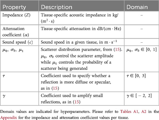
Table 1. List of properties assigned to tissues.

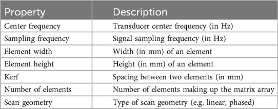
Table 2. List of parameters used to configure the transducer.

2.4 Simulation module

The goal of the simulation module (Figure 1C) is to generate view-dependent US images. This module is made of two parts.

The first part performs the ray tracing using OptiX. The goal of this module is to model large-scale effects (reflections, refractions and attenuation). This is done by computing, for each point along a scanline, the intensity I sent back to the transducer. The second part generates the US image by convolving the point spread function (PSF) with the scatterer distribution while taking into account the corresponding intensity I(l) along the scanline.

2.4.1 Background 2.4.1.1 Ultrasound physics

Here we first describe the phenomena happening during ray propagation: The wave loses energy due to attenuation following I(l)=I0e−lfα, with I0 the initial wave intensity and l the distance travelled in a given medium with attenuation α at frequency f. When it reaches a boundary, it is partially reflected and transmitted depending on the difference in impedance between the two media. The reflection and transmission coefficients R and T are written following Equations 1, 2:

R(Z1,Z2,θ1,θ2)=(Z2cos⁡(θ2)−Z1cos⁡(θ1)Z2cos⁡(θ2)+Z1cos⁡(θ1))2(1)

T(Z1,Z2,θ1,θ2)=1−R(Z1,Z2,θ1,θ2)(2)

cos⁡(θ1)=n→⋅v→(3)

cos⁡(θ2)=1−(Z1Z2)2(1−cos2(θ1))(4)

Where Z1 and Z2 are the impedances of the media at the boundary. θ1 computed following Equation 3, is the angle between the incident ray v→ and the surface normal n→. Finally, θ2 is the refracted angle and computed following Equation 4.

2.4.1.2 Rendering equation

When the wave propagates in tissue, it can encounter several boundaries and bounce multiple times, depending on the scene geometry. Hence, retrieving the total intensity at a given point P requires taking into account contributions coming from multiple directions. The field of computer graphics has faced similar challenges to compute global illumination.

We take inspiration from the rendering equation (30):

LP→ν=OP→ν+∫ΩfP,ω→νLP←ωcos⁡(θ)dω(5)

where:

• Ω is the surface hemisphere around the surface normal at point P.

• LP→ν is the amount of light leaving point P in direction ν.

• OP→ν is the light emitted at P in direction ν.

• fP,ω→ν is a Bidirectional Scattering Distribution Function (BSDF) giving the amount of light sent back by a given material in direction ν when it receives light from direction ω at point P.

• LP←ω is the amount of light received by P in direction ω.

• Finally, θ is the angle between the surface normal at P, nP→ and the incoming light direction ω.

2.4.2 Model derivation

Several modifications are made to adapt Equation 5 to US physics. Firstly, the term OP→ν is zero in our case as scatterers do not emit echoes.

We can then refer to the intensity sent back to the transducer from P as ITr. This term depends on the intensity I(P) arriving at P, expressed following Equation 6:

I(P)=∫ΩIP′→ωAP′→Pdω(6)

This represents the accumulation of echoes reaching P along directions ω from several points P′ located on other boundaries in the scene. This is illustrated in Figure 3 where contributions from P3 and P2 are gathered at P. IP′→ω is the intensity leaving P′ in direction ω and AP′→P is the attenuation affecting the wave from P′ to P along ω (denoted as ∼α− in Figure 3). IP′→ω depends in turn on the intensity accumulated at P′ (illustrated by incident rays at P1⋯P3 in Figure 3) following Equation 7:

IP′→ω=I(P′)fP′,ω′→ωcos⁡(θ′)(7)

With θ′ the angle between the incident ray ω′ and nP′→, and fP′,ω′→ω=R(Z1,Z2,ω′,ω)βT(Z1,Z2,ω′,ω)1−β where β is a binary variable equal to one when the ray is reflected, and zero otherwise. We randomly choose whether to reflect or refract a ray and β=1 when u<R(Z1,Z2,θ1,θ2), with u∼U(0,1), otherwise β=0. Here f is analogous to the BSDF in rendering and the corresponding loss of energy is represented at boundaries by |−| in Figure 3.

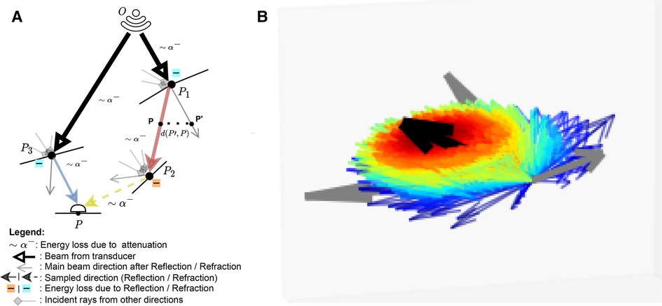
Figure 3. (A) A summary of the Monte Carlo path tracing logic: For a given point P in the scene, we integrate the contributions from multiple waves reaching P over its surface hemisphere. (B) A visualisation of the sampling pdf at intersections. The black arrow is analogous to the main beams in (A). Directions close to the main beam (e.g. ray leaving P1 in (A) have a higher chance of being sampled (thick red arrow) than the ones far from it (thick blue arrow, e.g. ray leaving P3 in (A). (A) Path tracing logic and (B) Ray distribution at intersection.

As we now have an expression for I(P), we can compute ITr. This term depends on whether or not P lies on an organ’s surface. The two cases are described below:

• Similarly to Burger et al. (15), on a boundary, the intensity reflected to the transducer ITr(P)=IR(P) is written following Equation 8:

IR(P)=(Z2−Z1Z2+Z1)2I(P)τcos⁡(θ)γ(8)

• Otherwise, it is simply equal to I(P) as shown in Equation 9:

ITr(P)=I(P)(9)

For a given point along a scanline with radial, lateral and elevation coordinates (r,l,e), the expression for the received echo is described by Equation 10:

E(r,l,e)=ITr(r,l,e)ρ(r,l,e)⊗T(r,l,e)(10)

where ρ(r,l,e) is a cosine modulated PSF and T(r,l,e) the scatterer distribution. Their expressions are given in Equations 11, 12, respectively.

ρ(x,y,z)=exp⁡(−12(r2σr2+l2σl2+e2σe2))cos⁡(2πfr)(11)

T(r,l,e)=∑q=1Nwqaqδ(r−rq)(12)

N is the number of scatterer