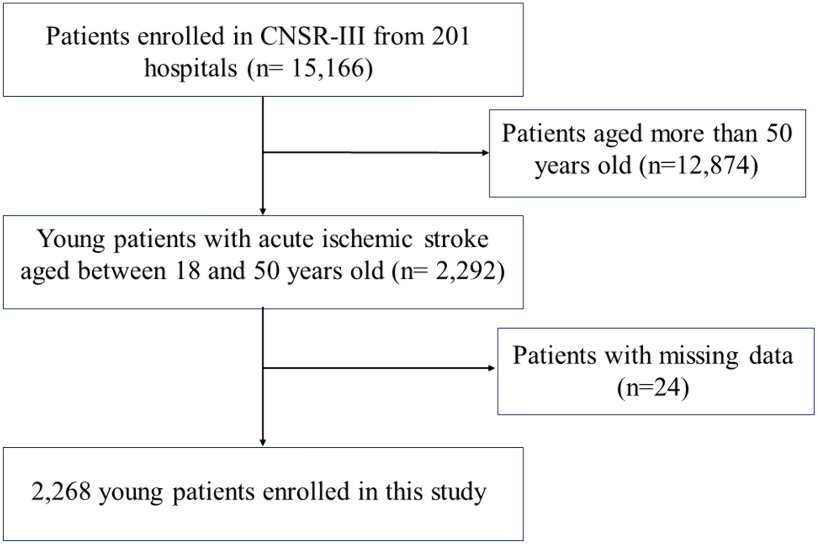
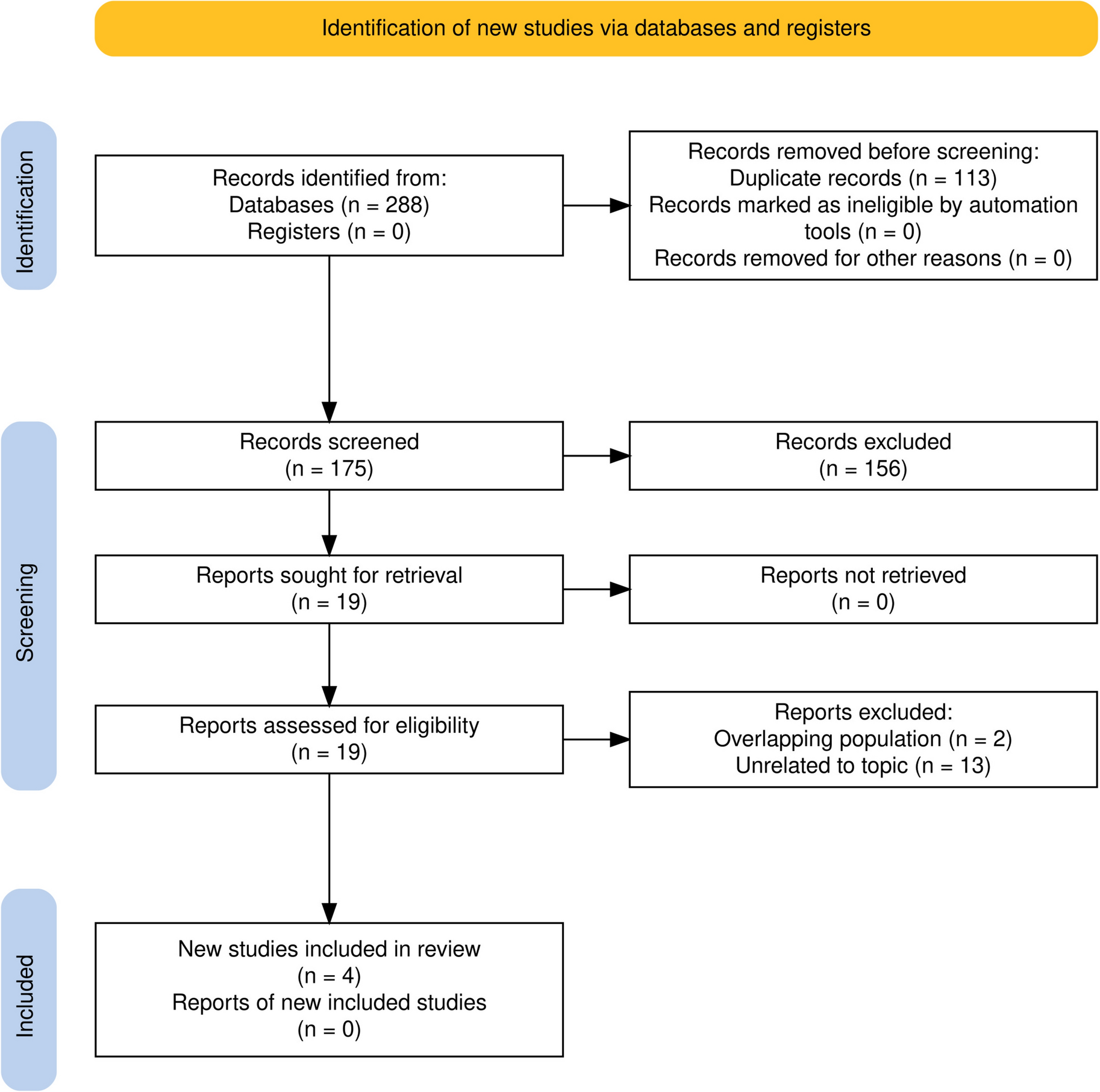
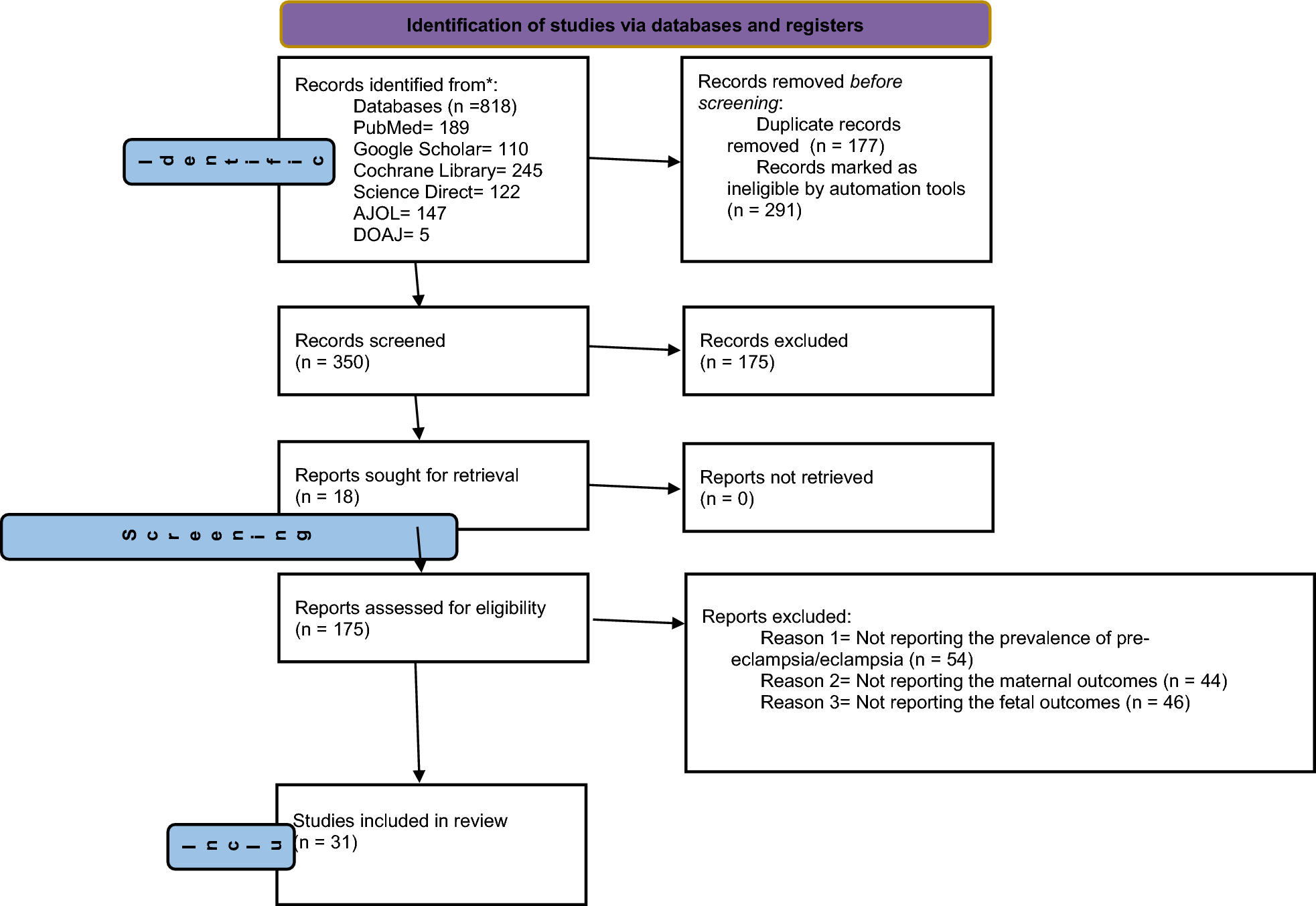
The clinical data for the 688 patients diagnosed to have SCLC during the study period were collected retrospectively. According to the enrollment and preliminary exclusion criteria, 260 patients with data sufficient to determine TSR were included, 25 of whom were excluded because their history of surgery and assessment had exceeded 4 months. Finally, data for 235 patients were included. Based on ROC curve analysis, the TSR cutoff was set as − 6.6%. Accordingly, the 235 patients were assigned to a responder group (TSR < − 6.6%, n = 119) or a non-responder group (TSR ≥ − 6.6%, n = 116) (Fig. 2).

Flowchart showing the patient selection process. R, ratio; SCLC, small-cell lung cancer; SR: shrinkage rate; TSR: tumor shrinkage rate

The baseline characteristics of the two groups are described in Table 1. There were no significant between-group differences in baseline characteristics, except for initial response to treatment and history of radiotherapy. Most of the enrolled patients were younger than 70 years and 85% were men. Approximately 91% of the patients had an ECOG score of 0–1. Most patients were heavy smokers, and 54% had ED-SCLC. For most of the eligible patients (77%), the first-line treatment was based mainly on the cisplatin + etoposide regimen, with a minority receiving a cisplatin + etoposide or irinotecan + cisplatin regimen. There was a significant between-group difference in the initial response to treatment (P < 0.001).

According to their disease stage, the 235 patients were divided into an ED-SCLC group and an LD-SCLC group for survival analysis (Supplementary Fig. 1A, B). Median OS was 15.80 months in both groups. PFS was approximately 1 month longer in the LD-SCLC group than in the ED-SCLC group (7.67 months vs. 6.87 months, P = 0.01) (Supplementary Fig. 1B).

Kaplan–Meier survival curve analysis showed that the median OS was 7.7 months longer in the responder group than in the non-responder group (20.00 months vs. 12.33 months; hazard ratio [HR] 0.55, 95% confidence interval [CI) 0.38–0.78, P < 0.0001) (Fig. 3A), as was median PFS (8.57 months vs. 5.07 months, HR 0.47, 95% CI 0.35–0.63, P < 0.0001) (Fig. 3B), indicating that the prognosis of the enrolled patients was predicted more accurately by our research method than by the traditional method.

Kaplan–Meier curves showing A OS and B PFS in the group with a TSR of < − 6.6% and the group with a TSR of ≥ − 6.6%. C Kaplan–Meier curves showing C OS and D PFS in patients with ED-SCLC in the group with a TSR of < − 6.6% and the group with a TSR of ≥ − 6.6%. D Kaplan–Meier curves showing PFS in patients with ED-SCLC in the group with a TSR of < − 6.6% and the group with a TSR of ≥ − 6.6%. E Time-dependent ROC curves for OS and the TSR in patients with SCLC. F Time-dependent ROC curves for PFS and the TSR in patients with SCLC. G Time-dependent ROC curves for OS and TSR in patients with ED-SCLC. H Time-dependent ROC curves for PFS and the TSR in patients with ED-SCLC. Kaplan–Meier curves for I OS and J PFS in patients with ED-SCLC in groups with a TSR of ≤ − 9%, a TSR of − 9% to − 4%, and a TSR of > − 4%. Kaplan–Meier curves for K OS and L PFS in patients with ED-SCLC in groups with a TSR of ≤ − 10%, a TSR of − 10% to − 6.6%, a TSR of − 6.6% to − 4%, and a TSR of > − 4%. ED-SCLC: extensive-disease small-cell lung cancer; OS: overall survival; PFS: progression-free survival; ROC:receiver-operating characteristic; SCLC: small-cell lung cancer; TSR: tumor shrinkage rate

Kaplan–Meier analysis was also used to examine differences in survival between responders and non-responders in the LD-SCLC group and the ED-SCLC group. In the LD-SCLC group, the OS curves for the responder and non-responder groups intersected, with a median OS of 16.03 months and 16.14 months, respectively (P = 0.17) (Supplementary Fig. 1C); however, there was a significant difference in PFS between the two groups (8.3 months vs. 6.2 months, P = 0.04) (Supplementary Fig. 1D), suggesting that our research method was more effective for prediction of PFS than for OS in patients with LD-SCLC. In the ED-SCLC group, median OS was approximately 13 months longer in the responder group than in the non-responder group (23.33 months vs. 10.20 months, P < 0.0001) (Fig. 3C). Median PFS was 8.57 months in the responder group and 3.90 months in the non-responder group (hazard ratio 0.28, 95% CI 0.17–0.44, P < 0.0001) (Fig. 3D).

To evaluate the prognostic value of our method, we then calculated the AUC for OS of < 6, < 12 and < 18 months and PFS of < 3, < 6 and < 12 months using ROC curves. For OS, the 12-month and 18-month AUCs were significantly lower than the 6-month AUC in patients with SCLC and in those with LD-SCLC (0.717 and 0.679 vs 0.895, Fig. 3E; 0.581 and 0.580 vs 0.915, Supplementary Fig. 1E). There was no obvious difference in the AUC for OS at 6, 12, or 18 months in patients with ED-SCLC (Fig. 3G). For PFS, the AUCs for all patients with SCLC and those with LD-SCLC decreased gradually between 3 and 12 months (0.927 vs 0.831 vs 0.679, Fig. 3F; 0.941 vs 0.753 vs 0.592, Supplementary Fig. 1F). In contrast, there were little difference in the AUCs between 3 and 12 months in patients with ED-SCLC (Fig. 3H). Overall, the ROC curves confirmed that our research method was well able to estimate the probabilities of OS and PFS, especially comparatively short survival and when applied to patients with ED-SCLC.

The above findings established the value of the TSR in patients with ED-SCLC and indicated that for these patients, stratification using − 6.6% as the TSR cutoff could better predict the prognosis than dividing patients into LD-SCLC and ED-SCLC groups. A smaller TSR value was associated with a better prognosis. Next, the patients with ED-SCLC were sub-grouped further according to various TSR values. Taking TSRs of − 9% and − 4% as the cutoffs, the patients were divided into three groups. The three survival curves were well separated for these patients. Median OS was 32.7 months for patients with a TSR of ≤ − 9%, 13.9 months for those with a TRS of 9% to − 4%, and 8 months for those with a TSR > − 4% (Fig. 3I); median PFS was 8.7, 6.6, and 3.2 months, respectively (Fig. 3J). Next, taking TSR values of − 10%, − 6.6%, and − 4% as the cutoffs, the patients with ED-SCLC were divided into four groups for survival analysis. Median OS was 32.7 months for a TSR ≤ − 10%, 15.9 months for a TSR of 10% to − 6.6%, 11.1 months for a TSR of − 6.6% to − 4%, and 8 months for a TSR > − 4%. The four OS curves were significantly different (Fig. 3K). In contrast, there was no significant difference in median PFS among the four groups, the value being 8.8 months for a TSR of ≤ − 10%, 8.6 months for a TSR of − 10% to − 6.6%, 5.1 months for a TSR of − 6.6% to − 4%, and 3.2 months or a TSR of > − 4%. This finding suggested that for PFS, there was no need to divide the patients with TSR values < − 6.6% into groups (Fig. 3L).

We then investigated the patients who had SCLC without brain metastasis. Fifty-nine of the 235 study participants did not have brain metastasis at diagnosis based on computed tomography and magnetic resonance scans but developed brain metastasis during treatment. The 59 patients were divided into LD-SCLC and ED-SCLC groups. However, as shown in Fig. 4A, the curves intersected, so we were unable to use this classification method to predict the prognosis of patients with SCLC and brain metastasis. Next, we used our nomogram method to analyze the relationship between the various TSRs and the prognosis of these patients. According to the survival analysis, the median BFS was 9.50 months in the responder group and 5.97 months in the non-responder group (P = 0.022) (Fig. 4B). We also grouped patients with LD-SCLC or ED-SCLC and brain metastasis by various TSR values and found that the survival curves of the two groups intersected (Fig. 4C, D). Median BFS in patients with LD-SCLC and brain metastasis was 9.67 months in the responder group and 8.63 months in the non-responder group, and was 8.79 months and 5.45 months, respectively, in patients with ED-SCLC and brain metastasis.

A Kaplan–Meier curves for BFS in patients with LD-SCLC and ED-SCLC. B Kaplan–Meier curves for BFS in patients with SCLC in a group with a TSR of < − 6.6% and a group with a TSR of ≥ − 6.6%. C Kaplan–Meier curves for BFS in patients with LD-SCLC in a group with a TSR of < − 6.6% and a group with a TSR of ≥ − 6.6%. D Kaplan–Meier curves for BFS in patients with ED-SCLC in a group with a TSR of < –6.6% and a group with a TSR of ≥ − 6.6%. E Kaplan–Meier curves for BFS in patients with ED-SCLC in a group with a TSR of ≤ − 9%, a group with a TSR of − 9% to − 4% and a TSR of > − 4%. F Kaplan–Meier curves for BFS in patients with ED-SCLC in a group with a TSR of < − 10%, a group with a TSR of − 10% to − 6.6%, a group with a TSR of − 6.6% to − 4%, and a group with a TSR of > − 4%. BFS, brain metastasis-free survival; ED-SCLC: extensive-disease small-cell lung cancer; LD-SCLC: limited-disease small-cell lung cancer; SCLC: small-cell lung cancer; TSR: tumor shrinkage rate

Using TSR values of − 9% and − 4% as the cutoffs, we then divided the patients with ED-SCLC and brain metastasis into three groups. Median BFS was 8.67 months for a TSR of ≤ − 9%, 8.6 months for a TSR of − 9% to − 4%, and 4.2 months for a TSR of > − 4%. As shown in Fig. 4E, the curves for the TSR ≤ − 4% and TSR > − 4% groups were clearly separated. However, when we divided the same patients into four groups, as shown in Fig. 4F, there was a difference in median BFS between the TSR ≤ − 4% and TSR > − 4% groups. Therefore, for patients with ED-SCLC and brain metastasis, stratification using a TSR cutoff of − 4% could better predict the prognosis than stratification using a TSR cutoff of − 6.6%.

The recurrence pattern after failure of the first-line treatment of SCLC was mainly relapse of the primary lesion (31%), followed by brain metastasis (17%), lung or pleural metastasis (7%), bone metastasis (7%), liver metastasis (7%), mediastinal or cervical LNM (6%), adrenal metastasis (4%), intra-abdominal LNM (1%), pancreatic and intestinal metastasis (2%), and unknown (18%) (Fig. 5).

Disease recurrence patterns

Using the univariate and multivariate Cox proportional hazards models, we analyzed the associations of PFS and OS with the patients’ clinical characteristics, including age, sex, smoking status, body mass index, ECOG score, TNM stage, treatment regimen, history of radiotherapy, and tumor burden. The univariate Cox proportional hazards model showed a correlation of smoking ≥ 20 packs/year with PFS, with an increase in risk of 44% (HR 1.44, 95% CI 1.03–2.02, P = 0.035), and a correlation of M1 stage with PFS, with an increase in risk of 46% (HR 1.46, 95% CI 1.09–1.95, P = 0.01). Furthermore, age older than 70 years was an indicator of poor OS, with an increase in risk of 58% (HR 1.58, 95% CI 1.10–2.29, P = 0.015). Previous radiotherapy was an indicator of favorable OS, with a decrease in risk of 33% (HR 0.67, 95% CI 0.47–0.96, P = 0.03). No other patient factor had a significant correlation with PFS or OS (Table 2). The multivariate Cox proportional hazards model revealed that M stage had an impact on PFS, while age, prior radiotherapy, and tumor burden had an impact on OS (Table 3).

Based on previous work, we constructed a nomogram combining age, radiotherapy, tumor burden, and the TSR that was able to predict OS of > 6 months, > 12 months and > 18 months (Fig. 6A) and a nomogram combining M stage and TSR that was able to predict PFS > 3 months, > 6 months, and > 12 months (Fig. 6B). We evaluated the predictive performance of the nomogram using a calibration curve, which showed good agreement between the predicted probability of the nomogram and the actual probability (Fig. 6C, E). Next, decision curve analysis was used to explore the clinical utilization of the nomograms. Figure 6D, F shows the results of the decision curve analysis for the two models (nomogram model and shrinkage rate) when applied to OS and PFS. In comparison with the shrinkage rate, the nomogram model had higher net benefit in prediction of which patients should receive more aggressive treatment. This finding suggested that the nomogram combining traditional diagnostic factors and the shrinkage rate has better predictive power than the shrinkage rate alone.

A Nomogram to determine the probability of OS for > 6 months, > 12 months, and > 18 months. B A nomogram to determine the probability of PFS for > 6 months, > 12 months, and > 18 months. B Value of each risk factor can be converted into a corresponding score according to the “points”. After adding up the individual risk scores for these risk factors, draw a line descending from the axis labeled “Total points” until it intercepts each clinical predictive score for SCLC. C Calibration curves for the OS nomogram at 6, 12, and 18 months. E Calibration curves for the PFS nomogram at 3, 6, and 12 months. Results of DCA for two models (the nomogram model and shrinkage rate) applied to OS (D) and PFS (F), respectively. The DCA curves measure the net benefit (y-axis) versus the model’s high risk threshold (x-axis) for the different models. DCA: decision curve analysis; OS: overall survival; PFS: progression-free survival; SCLC: small-cell lung cancer