1 Introduction

In recent years, there has been extensive research on neural networks that aim to mimic the human brain. Notably, in fields like image classification and object recognition, state-of-the-art neural networks such as YOLO (Redmon et al., 2016) and Vision Transformer (ViT) (Dosovitskiy et al., 2020) have demonstrated remarkable performance, surpassing even human discrimination capabilities.

Most widely used neural networks today are based on the formal neuron model, forming what is known as Artificial Neural Networks (ANNs) (Hopfield and Tank, 1985; Dong et al., 2021; Sharifani and Amini, 2023). As show in Figure 1A, ANNs employ the formal neuron model to calculate the weighted sum of inputs, followed by a non-linear activation function like ReLU or Sigmoid. Typically, activations and weights are represented as single-precision floating-point or 8-bit integer values. While the energy required for each multiplication may seem negligible at around 0.2 pJ per operation with 8-bit precision (Courbariaux et al., 2016), modern neural networks consist of millions of neurons, resulting in significant overall energy consumption during inference (Bernstein et al., 2021). Therefore, reducing the energy required for multiplications is crucial to minimize power consumption during neural network inference.

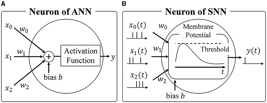
Figure 1. (A) Neuron of ANN, (B) Neuron of SNN.

Spiking Neural Networks (SNNs) (Maass, 1997; Taherkhani et al., 2020; Nunes et al., 2022; Eshraghian et al., 2023) have gained attention as an alternative to ANNs. As shown in Figure 1B, SNNs emulate the biological brain's functionality, representing activations as spike trains comprising binary spike states (spike firing or absence of firing). This sparse spike representation offers two advantages when considering hardware accelerators. Firstly, the expensive integer or floating-point multiplications in ANNs can be replaced with additions. Unlike ANNs where activations are multiplied by synaptic weights, SNNs track changes in membrane potential by simply adding the synaptic weight upon receiving a spike event, as spikes are binary. Secondly, SNNs only require updating membrane potentials when they receive spikes, aligning well with asynchronous circuits and further reducing energy consumption. Leveraging the sparsity of spike events and event-driven computation, SNNs offer exceptional power efficiency, making them a preferred choice for neuromorphic architectures. Notably, IBM's TrueNorth (Akopyan et al., 2015) and Intel's Loihi (Davies et al., 2018) are hardware accelerators designed specifically for SNNs, successfully achieving significant energy reductions through asynchronous communication.

In addition to their low energy consumption, the learning algorithms for SNNs have dramatically improved in recent years. One such algorithm is the Surrogate Gradient (SG) method, which treats the non-differentiable spikes as differentiable smooth functions, allowing the SNN to be treated as a Recurrent Neural Network (RNN) and learned through Backpropagation through time (BPTT) algorithm. However, because the BPTT unfolds the SNN in the time direction for learning, the gradient propagates in the time direction, extending the propagation distance of the gradient. This can easily cause gradient vanishing/explosion, making it difficult to achieve sufficient inference performance in large-scale neural networks (Zenke and Vogels, 2021; Sun et al., 2022; Guo et al., 2023). Therefore, the ANN-SNN conversion, which maps the parameters learned by the ANN to the SNN, has been developed, making it possible to infer the SNN while maintaining the same accuracy as the ANN (Sengupta et al., 2019; Hu et al., 2021). The accuracy of models trained with each method using the CIFAR-10 dataset is shown in Table 1. From Table 1, it can be seen that when the parameters of the SNN are determined by the ANN-SNN conversion, inference performance comparable to that of the ANN can be achieved, but the performance obtained by the SG method is significantly inferior compared to the ANN. The ANN-SNN conversion is also used for complex tasks other than class classification, such as object detection. Kim et al. (2020) showed that by converting YoLo to SNN, an energy efficiency 280 times that of the ANN implementation can be achieved.

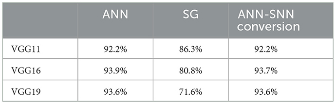
Table 1. Inference accuracy of models trained with SG and ANN-SNN conversion.

Despite the superior characteristics of SNNs over ANNs, there is still potential for energy and latency reduction. SNNs rely on spike firing probabilities to represent information, necessitating sufficiently long spike firing sequences to accurately measure these probabilities.

In this paper, we propose a method to reduce inference energy and latency in SNNs based on Bayesian fusion. Spikes can be represented as binary variables indicating firing or non-firing states. The observed number of spike firings in a given time period can be modeled using a binomial distribution. In other words, decoding information represented by a spike firing sequence is equivalent to determining the most probable parameters of the binomial distribution that generated the observed spike firing sequence. In general, there is a trade-off between inference accuracy, latency, and energy consumption. Longer observation of spike firing sequences allows for higher accuracy in parameter estimation but increases latency and reduces energy efficiency. In this study, we reduce energy consumption and latency while maintaining inference accuracy by compensating for information degradation resulting from shortened spike sequence observations using prior knowledge about spike firing probabilities. Specifically, we predict the probability of firing for neurons in the final output layer based on the firing sequences of neurons in the shallow layers of the network. We employ Bayesian fusion with the firing sequences observed in the final output layer to reduce the required length of spike firing sequence observations without compromising the accuracy of firing probability estimation. Numerical experiments utilizing VGGs and ResNets demonstrate that we can achieve up to 48.0% energy reduction while maintaining inference accuracy in image classification tasks involving MNIST, CIFAR-10, and CIFAR-100 datasets.

2 Related works 2.1 Enhancing inference efficiency in SNN

Research focused on reducing the inference time steps of Spiking Neural Networks (SNNs) converted from Artificial Neural Networks (ANNs) is actively pursued (Hwang et al., 2021; Bu et al., 2023; Rathi and Roy, 2023). Various techniques for converting ANNs into efficiently inferable SNNs have been proposed, such as Robust Normalization (Rueckauer et al., 2017) RTS (Deng and Gu, 2021) and RMP (Han et al., 2020). Methods addressing the discrete spike sequences of SNNs include using clip functions or quantized ReLU functions instead of ReLU during pre-conversion training, as seen in TCL (Ho and Chang, 2021) and QCFS (Bu et al., 2023). Innovations applied directly to SNN neuron models, like the “reset-by-subtraction” method for resetting neuron firing potentials, minimize information loss compared to resetting methods that force the membrane potential to zero, thereby enabling faster inference (Diehl et al., 2015; Hwang et al., 2021; Rathi and Roy, 2023).

Apart from techniques for converting to efficiently inferable SNNs, strategies to enhance network structure for reducing inference time have also been proposed. For example, the early exit model outputs the final classification result from shallow layers without waiting for deeper layer results when input classification is straightforward (Chen et al., 2023; Li Y. et al., 2023). This model incorporates an internal classifier (IC) that predicts the final output from activations in internal layers of a multi-layer neural network (Li C. et al., 2023). In this approach, inference terminates early and outputs the final prediction once the confidence in predictions from the IC exceeds a predefined threshold.

Traditionally, methods have primarily focused on early termination or reduction of inference time in the final classifier layer, switching between early termination based on confidence in the IC or final classifier (FC), limiting accuracy to the precision of the IC or FC alone. Therefore, the proposed method achieves higher performance by statistically integrating outputs from both intermediate and final classifiers, surpassing what a single classifier can achieve.

2.2 Hardware accelerator for SNN

The sparse representation of spikes suits well with hardware, and a variety of SNN chips have been proposed, led by IBM's TrueNorth. TrueNorth is a highly specialized processor that can handle a specific model of spiking neurons (Akopyan et al., 2015). TrueNorth consists of 4,096 cores, each of which has a crossbar consisting of 256 axons and 256 neurons. The cores are connected to each other by a two-dimensional mesh network, and any neuron can be connected to any axon. In order to reduce the circuit size of the neurons, a virtual neuron scheme is adopted where a single neuron circuit is time-shared. Each neuron in TrueNorth uses an event-driven circuit that updates the membrane potential upon receiving a spike, which has succeeded in significantly reducing power consumption. For example, the TrueNorh chip, manufactured in a 28 nm process, uses 5.4 billion transistors, yet requires only 63 mW to recognize a 400 × 240 pixel image input at 30 FPS. The energy consumption per spike ignition is 26 pJ.

Another SNN accelerator is the SpiNNaker (Merolla et al., 2014) being developed at the University of Manchester, which consists of 18 ARM9s, a lightweight general-purpose processor core developed by ARM, and a dedicated processor that handles the interprocessor connections. In contrast to TrueNorth, which specializes in efficient simulation of integrate-and-fire models, SpiNNaker, which uses general-purpose processors, can run arbitrary neuron models. In addition, SpiNNaker can efficiently transfer spike information through multicast communication, and a single board with 48 chips can simulate a neural network of 250,000 neurons and 80 million synapses in real time.

Table 2 summarizes the differences between ANNs and SNNs.

Table 2. Comparison of ANN and SNN.

3 Preliminary 3.1 Artificial neural network

Each neuron in the ANN takes the product of the input activation x and the synaptic coupling weights w, and adds a bias b. This is then passed through a nonlinear function f to obtain the output activation y as follows Equation (1):

y=f(∑i=1nwixi+b).    (1)

Activation values are often represented by single-precision or half-precision floating-point numbers, or by 8-bit integers.

In ANN, when the parameters of one layer change during training, the input distribution for the subsequent layers changes. Since this change increases as the layer depth increases, it is difficult to take a large learning rate in order to suppress learning divergence, which is known to be a “covariate shift” problem. To solve this problem, the Batch Normalization (BN) technique has been proposed (Ioffe and Szegedy, 2015). BN normalizes the input of the layers in each mini-batch to have mean 0 and variance 1, followed by scaling and biasing processes using learnable scaling factors and bias parameters. More specifically, the operation of BN layer is represented as follows Equation (2):

y′=γy-μσ2+ϵ+β,    (2)

where μ and σ2 are the mean and variance for each mini-batch, respectively, and γ and β are the learnable scaling factor and bias parameter. Since μ, σ2, γ, and β are fixed and treated as constants during inference, the batch normalization layer can be fused into the previous linear layer during inference to reduce the number of operations. Specifically, they can be integrated into the weights of the previous layer, as shown in Equations (3, 4).

b^=γσ(b-μ)+β    (4) 3.2 Spiking neural network

The biological brain is believed to represent information by transient voltage signals called spike firing, and a computational model that mimics this mechanism is called the spiking neural network (SNN). In this study, we use the integrate-and-fire (IF) model, which is considered to be the most popular model and has been proposed in many hardware implementations. In the IF model, a neuron is represented as a node with a membrane potential as its internal state. When a neuron receives a spike from another neuron, it updates its membrane potential according to the synaptic connection weights between it and that neuron. This behavior can be described as follows:

Vit=Vit-1+∑jwijVthΘjt+bi,    (5)

where Vit is the membrane potential of neuron i at time t, wij is the synaptic weight from i-th neuron to j-th neuron, Vth is the threshold voltage, and bi is the bias value of the i-th neuron. Θjt is a binary variable that represents the presence or absence of spike firing of j-th neuron at time t. This is a binary variable that represents the presence or absence of spike firing in j-th neuron at time t, and is calculated from the membrane potential of j-th neuron as follows:

Θjt={1Vjt>Vth0otherwise.    (6)

Each neuron resets its membrane potential after firing a spike. There are two methods of resetting the membrane potential: setting the membrane potential to zero or subtracting the threshold voltage. The latter method is known to cause less information degradation (Rueckauer et al., 2017), so we adopt the latter method in this study. The method is described as follows:

Vit=Vit-VthΘit.    (7)

Combining Equations (5–7), we can derive an update rule for the membrane potential of the ith neuron in the lth layer as:

Vl,it=Vl,it-1+∑jwijVthΘl-1,jt+bi-VthΘl,it.    (8) 3.3 ANN-to-SNN conversion

While information transfer using binary spikes greatly improves the energy efficiency of SNNs, it also makes learning by backpropagation, which requires gradient computation, difficult. There is some research using the STDP rule, which changes the synaptic connection weights according to the time difference between spikes, which is considered to be one of the basic learning algorithms of the biological brain (Bi and Poo, 1998). However, its application is limited to simple tasks such as MNIST, and it is still difficult to perform very complex tasks such as those realized by modern DNNs (Diehl and Cook, 2015). To solve this problem, a method was proposed to convert the weights learned in the ANN to SNNs and only perform inference in SNNs (Rueckauer et al., 2017). The basic principle of converting ANNs into SNNs is to match the output activity value of ReLU with the firing rate of spiking neurons. To obtain the conversion equation from ANN to SNN, we first accumulate (Equation 8) over the simulation timestep from time 1 to T, divide both sides of the equation by T, and yield Equation (9):

Vl,itT=Vl,i0T+∑j=1Nwij∑t=1TVthΘl-1,jtT+bi-Vth∑t=1TΘl,itT.    (9)

Let pl,i=∑t=1TΘl,it/T be the spike firing probability of the i-th neuron in the l-th layer, and written as:

pl,i=1Vth(∑j=1Nwi,jVthpl-1,j+bi-Vl,it-Vl,i0T).    (10)

From Equation (10), it can be inferred that the spike firing rate is proportional to the weighted sum of the input spike firing rate, excluding (Vl,it-Vl,i0)/T. Note that the membrane potential has an initial value at t = 0, whereas spikes are observed starting from t = 1.

4 Error analysis of converted SNN

In order to improve the energy efficiency of SNNs, it is important to first analyze the error factors in detail. To this end, we firstly classify the error factors into two types: errors that are incurred during the ANN to SNN conversion process and those incurred when decoding the spike firing representation of the information.

4.1 Errors induced during ANN to SNN conversion process

The error El, i in the ANN-SNN conversion can be calculated as the difference between the activation value yl, i of the ANN and the firing rate Vthpl, i of the SNN scaled by the threshold, i.e., El, i = yl, i−Vthpl, i. The application of the ANN-SNN conversion assumes the use of the ReLU function as the activation function of the ANN, and El, i is given by Equation (11):

El,i   =  ReLU(∑j=1nwi,jyl−1,j+bi)         −(∑j=1Nwi,jVthpl−1,j+bi−Vl,it−Vi,i0T)    (11)

where yl, i represents the activation value of neuron i in layer l and T represents a simulation timestep, which is a positive integer. If the input to the ReLU function, ∑j=1nwi,jyl-1,j+bi, is positive, El, i is given by

El,i=∑j=1Nwi,j(yl-1,j-Vthpl-1,j)+Vl,it-Vl,i0T.    (12)

Noting that yl−1, j−Vthpl−1, j = El−1, j, this equation can be further written as Equation (13):

El,i=∑j=1Nwi,jEl-1,j+Vl,it-Vl,i0T.    (13)

This shows that the error in the activation values of the ANN and SNN at layer l is the sum of the weighted errors at layer l−1 plus (Vl,it-Vl,i0)/T. On the other hand, if the input to the ReLU function, ∑j=1nwi,jyl-1,j+bi, is negative, the neuron does not fire, pl, i = 0, and therefore El, i = 0.

The error E1, i at the input layer depends on the coding scheme of the input. In SNNs, a method called direct coding, which directly uses floating point values as the input to the first layer, is common, and in this case, E1, i = 0 (Rathi and Roy, 2023). Conventionally, the membrane potential Vl,i0 of the SNN is initialized to 0 and the threshold Vth is fixed at 1, so Equations (10, 12) can be simplified as follows Equations (14, 15):

pl,i=∑j=1Nwi,jpl-1,j+bi-Vl,itT    (14) El,i=∑j=1N(yl-1,j-pl-1,j)+Vl,itT.    (15)

In the following, we assume that the membrane potential Vl,i0 is initialized to 0 and the threshold Vth is fixed at 1.

According to Equation (15), we notice that the conversion of ANN to SNN induces an error term Vl,i(t)/T, which is inversely proportional to the integration time T. Although increasing T will decrease the estimation error, it will also increase the energy required for inference. Hence, there is a trade-off between inference accuracy and energy. We also notice that the spike firing probability pl, i is restricted to a range of [0, 1], whereas ANNs typically have no such constraints. For instance, if the threshold Vth is extremely high compared to the synaptic weights, it takes a long time for the membrane potential to reach Vth, resulting in a low spike firing probability. Conversely, if Vth is extremely small compared to the synaptic weight, the membrane potential will exceed Vth regardless of the spike input, which again causes information degradation.

Hence, synaptic weight Wl, i, j should be carefully normalized to avoid too low or too high spike firing probability. To this end, various data-driven normalization methods have been proposed (Cao et al., 2015; Diehl et al., 2015). One of the well-known methods is “layer-wise normalization” proposed by Diehl et al. (2015), where the synaptic weights are normalized so that the maximum activations calculated using the training dataset does not exceed Vth (i.e. 1.0). Hence, the synaptic weights wlSNN are calculated as follows:

wlSNN=λl-1λlwl,       blSNN=1λlbl,    (16)

where λl is the maximum activations in l-th layer calculated by using the training dataset. Later, a modified layer-wise normalization has been proposed, where λl is selected to be 99.9th percentile of the maximum activations to improve the robustness to outliers (Rueckauer et al., 2017). More recently, Kim et al. have proposed “channel-wise normalization” (Kim et al., 2020). In addition to this normalization, methods for reducing errors by adjusting the threshold have also been developed (Sengupta et al., 2019; Park et al., 2020).

Furthermore, techniques have been proposed to reduce SNN errors by pre-charging the initial membrane potential to promote early firing of the first spike (Hwang et al., 2021). Bu et al. (2023) demonstrated that neurons fire more uniformly by using floor and clipping functions instead of the ReLU function during ANN training and initializing the membrane potential to half of the threshold during SNN inference.

4.2 Error induced during decoding spike outputs

Since SNNs represent information in terms of spike firing frequency, the inference results of SNNs need to be decoded again into a continuous value representation. Let a