1 Introduction 1.1 Background

Epilepsy, a neurogenic disorder characterized by abrupt and transient disturbances in the body, manifests through sudden electrical bursts within the brain. These recurrent electrical discharges are commonly referred to as “epileptic seizures” or “ictal events” and more colloquially as “fits.” According to the survey, more than 50 million people worldwide are affected by epilepsy, representing approximately 2% of the global population (Moshé et al., 2015; World Health Organization, 2024). Consequently, the diagnosis of epilepsy is one of the utmost concerns. The most prevalent and reliable method for diagnosing epilepsy to date is recording the brain signals, primarily electroencephalography (EEG). Electrocorticography (ECoG) is also important and is particularly used for surgical intervention. Brain signals are primarily visually inspected by trained neuro-clinicians or neurophysiologists (Banerjee et al., 2009; Duque-muñoz et al., 2014). However, even standard EEG recordings for diagnosing epilepsy can last between 30 min to 6 h, rendering the visual scrutinization process very time-consuming. EEG data are often contaminated by motion artifacts, background noise, and interfering patterns from other neurological disorders. In developing countries, where the availability of neurophysiologists is low, diagnosing epilepsy using EEG becomes even more challenging and prone to manual errors (Banerjee et al., 2009). This situation makes the diagnosis of epilepsy using EEG very difficult and increases the likelihood of manual errors (Schuyler et al., 2007; Gandhi et al., 2010, 2012). Misdiagnosis of epilepsy often leads to the administration of improper drugs, which can prove to be life-threatening for patients. Hence, there is a dire need to develop an accurate, computationally fast, and robust tool for the diagnosis of epilepsy.

1.2 State-of-the-art

Significant research efforts have been dedicated to developing expert systems for the automated detection of ictal patterns or epileptic seizures in EEG. This section discusses some of the key findings reported in this area. Early breakthrough studies, such as those by Gotman (1999), relied on mimetic techniques that utilized descriptions provided by experienced neurophysiologists, including attributes such as crest, sharpness measures, time durations, inclinations, and more. However, this method proved to be inaccurate due to the heterogeneity among ictal patterns. Subsequent automated diagnosis methods for epilepsy involved the application of various frequency-domain techniques, such as the fast-Fourier transform (Polat and Güneş, 2007), and time-domain techniques, such as the empirical mode decomposition (Sharma and Pachori, 2015). Approaches based on FFT failed to capture the correct onset of ictal events due to their assumption of EEG as stationary despite its original non-stationary nature. The introduction of time–frequency domain techniques such as the short-time Fourier transform (Tzallas et al., 2009), especially wavelets (Gandhi et al., 2011; Swami et al., 2014; Faust et al., 2015; Edakawa et al., 2016; Swami et al., 2016a), aided in the development of many automated seizure detection models (Acharya et al., 2013).

Researchers have explored a wide variety of features for characterizing ictal patterns in EEG, including combinations of lower- and higher-order statistical parameters such as standard deviation (Gajic et al., 2015), kurtosis (Acharya et al., 2013), chaotic parameters such as correlation dimension and Lyapunov exponents (Tzallas et al., 2009; Acharya et al., 2013), Shannon entropy (Gandhi et al., 2011; Swami et al., 2017), energy (Swami et al., 2014, 2016a), and many more. Earlier, there was a general assumption that increasing the number of feature sets would improve the machine learning (ML) model’s accuracy. However, ample evidence suggests that increasing the dimensionality of the feature matrix could increase the computational cost of the expert system, while some features may even decrease the accuracy of the ML model. Hence, feature engineering for epilepsy diagnosis can present a paradox. Consequently, many researchers opt to exclusively utilize deep learning (DL)-based methods. While these methods perform optimally when trained with sufficiently large annotated/synthetic datasets (Pascual et al., 2020; Srinivasan et al., 2023; Dash et al., 2024), practical applications often encounter scarcity of such datasets and/or face challenges with the “black box” nature of the model. This opacity seldom instills confidence in clinicians to adopt new computer-aided diagnosis (CAD) systems. Therefore, identifying the underlying issues hindering the adoption of CAD in clinical settings is paramount.

1.3 Identification of problem statement and novelty

Some seminal research efforts on optimal feature selection have yielded noteworthy results (Gandhi et al., 2012). However, the majority of research endeavors focusing on feature optimization and selection have centered around a single objective function (Acharya et al., 2013; Dhiman and Saini, 2014; Dash et al., 2024), primarily aimed at enhancing the accuracy of expert systems. This often results in the development of models with either exceedingly slow computation times and high accuracy or rapid models with lower accuracy. Feature selection methods could provide a faster alternative (Nara et al., 2016; Krishnan et al., 2024); however, those methods usually do not solve multiple objectives. Additionally, the scalability issues of these models are frequently overlooked and often lead to the selection of a maximum number of features. This is an important issue for realizing practicability in clinical settings (Swami et al., 2018; Tirumani et al., 2018). A compromise between sensitivity and specificity rates has often been observed (Mormann et al., 2007; Swami et al., 2016a), rendering the replication and practical application of results in clinical settings challenging. The scarcity of extensive, annotated datasets further exacerbates these challenges. This research seeks to bridge the gaps between these extremes.

Moreover, much of the literature in epilepsy research lacks a clear delineation of the procedure for constructing optimization functions, hindering future replicable research. The present study aims to demonstrate the application of evolutionary transfer optimization (ETO) (Tan et al., 2021) through an evolutionary multi-objective optimization (EMO) approach. The transfer optimization methodology is employed to train specific datasets, with testing datasets consisting entirely of out-of-sample signals. In this context, the EMO method employed is the non-dominant sorting genetic algorithm (NSGA)-II, aimed at simultaneously minimizing the number of feature sets and error rates. The knowledge transfer is directed toward minimizing classification error rates while maximizing accuracy and minimizing features, aligning with the concept of Maximizing Accuracy while Minimizing Features (MAMF). This concept can also be applied to address a broad spectrum of not only neurological but also various real-life challenges.

1.4 Brief about the next sections

The following section of this article outlines the materials and methods employed. It comprehensively details the datasets utilized in this study and endeavors to present a procedural execution methodology for developing an expert system. Subsequently, the subsequent section of this article presents the results and discussion. Finally, the conclusions section summarizes the significant developments from this study and discusses its future scope.

2 Methods 2.1 Datasets

Datasets from three different repositories were used in this study. The first dataset is freely available in the epilepsy EEG repository of the University of Bonn (UoB) (Andrzejak et al., 2001). The datasets within this repository have become a common benchmark for validating expert systems for detecting epileptic seizures. The datasets considered from this database are named set C, set D, and set E. Each of these subsets consists of intracranial EEG, i.e., electrocorticography (ECoG) segments acquired with a sampling rate of 173.61 Hz from five epilepsy patients, with each segment comprising 4,097 samples lasting for a duration of 23.6 s. The signals in set C were acquired from the region around the hippocampus location opposite the hemisphere of the epileptogenic zone, while the signals in set D were acquired from the epileptogenic zone. Both sets C and D consisted of interictal (non-ictal) events, whereas only the signals in set E consisted of epileptic seizure (ictal) events.

The second dataset considered in this study is available from our repository (Swami et al., 2019). The signals in this repository were collected from 10 epilepsy patients using the Grass Telefactor Comet AS40 machine. The acquisition was conducted at the Neurology & Sleep Centre (NSC) by a trained clinician under the supervision of a neurophysiologist. During acquisition, gold-plated scalp EEG electrodes were positioned according to the international 10–20 electrode placement system. The data collected at 200 Hz from all channels were segmented into signals lasting for a duration of 5.12 s, comprising 1,024 samples. The subsets named interictal and ictal events were considered in this study.

The third dataset considered in this study was collected from the database of Sri Ganga Ram Hospital (SGRH). The signals downloaded from this repository were collected from 20 epilepsy patients (Gandhi et al., 2011, 2012; Swami et al., 2016a). The sampling rate during acquisition was fixed at 400 Hz, and the Grass Telefactor Twin3 EEG machine was used for acquisition. The data from all channels were segmented into signals lasting for a duration of 10 s, comprising 4,000 samples. The subsets with interictal and ictal stages were considered from this database.

Samples of EEG segments from each of the three repositories are shown in Figures 1–3.

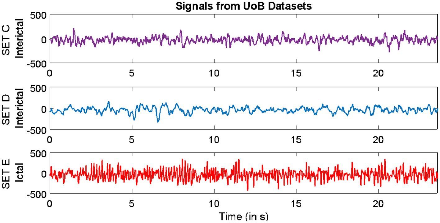
Figure 1. Example of signals from University of Bonn (UoB) datasets.

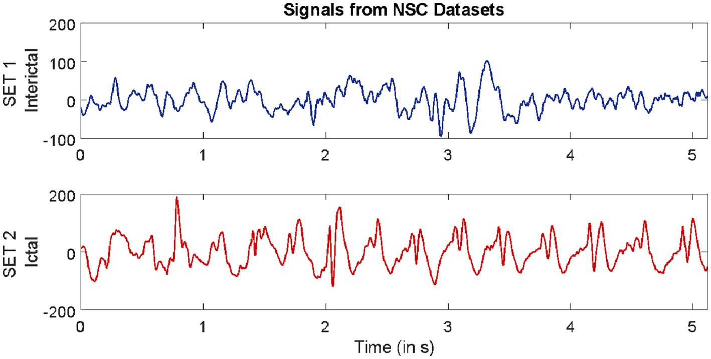
Figure 2. Example of signals from Neurology & Sleep Centre (NSC) datasets.

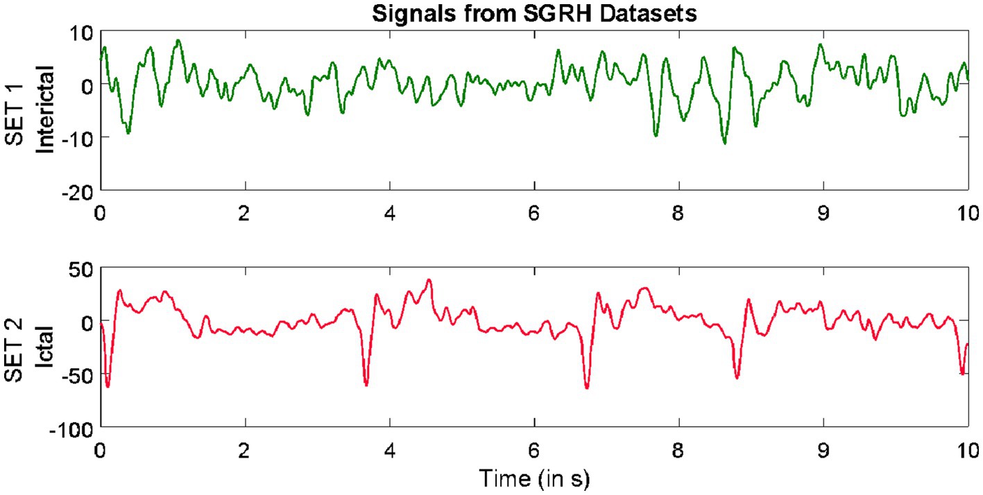
Figure 3. Example of signals from Sri Ganga Ram Hospital (SRGH) datasets.

2.2 Feature engineering

The process involves utilizing domain knowledge of the signals/datasets to extract a relevant set of attributes, referred to as features, which can then be fed into the ML classifier. The entire feature engineering procedure of this study is outlined as follows.

2.2.1 Multi-resolution analysis (MRA) using wavelet packet transform (WPT)

This involves selecting the most relevant wavelet transforms that could completely characterize the signal. The wavelet coefficients Wi with subspaces Si⊥Wi , i∈Z satisfying the multi-resolution analysis (MRA) conditions. Unlike discrete wavelet transform (DWT), the double-branched architecture of wavelet packet transform (WPT) provides a much smaller separation between the frequency bands and aids finer analysis. This technique has proven effective over DWT (Swami et al., 2017). The wavelet coefficients of the last decomposition level were stored for extracting features. For signal xn , an orthonormal basis of Wi can be given by Ψn , which is controlled by time shift and dilation parameters. Based on our previous findings (Gandhi et al., 2011), “Coiflets” mother wavelet with a single scaling function was selected in this study. The MRA using WPT was adopted in this study. In this method, a signal xn is passed through a series of quadrature mirror filters (Gandhi et al., 2012; Swami et al., 2015a, 2017). During this recursive process, details and approximations are fed into the next filters. The double-branched architecture of WPT is shown in Figure 4. As an example, the input signal with a sampling rate Fs=200 Hz is fed into the WPT architecture in Figure 4. Resampling all input signals to a uniform frequency guarantees that the feature extraction is conducted consistently across signals with identical spectral characteristics (Frølich et al., 2015). Thereby also ensuring knowledge transfer. After the signal is fed into the WPT architecture, the frequency band for the input signal range between 0−Fs/2 Hz. If we denote the wavelet coefficient by Wfl where, l is the decomposition level and f is the index of the frequency band, then the signals are decomposed/downsampled by 2 into the details W11 (i.e., approximation with frequency band between 0−Fs/4 Hz) and W21 (i.e., detail with frequency band between Fs/4−Fs/2 Hz after the first decomposition level). Similarly, after l = 2, the preceding W11 is decomposed into W12 (i.e., approximation with frequency band between 0−Fs/8 Hz) and W22 (i.e., detail with frequency band between Fs/8−Fs/4 Hz). In addition, the W21 is decomposed into W32 (i.e., approximation with frequency band between Fs/4−3Fs/8 Hz) and W42 (i.e., approximation with frequency band between 3Fs/8−Fs/2 Hz). This process was recursively continued till seventh decomposition level, thus generating 2l = 128 wavelet coefficients. It is very important that the length of the signal is sufficient to capture the ictal or non-ictal pattern (Behara et al., 2016).

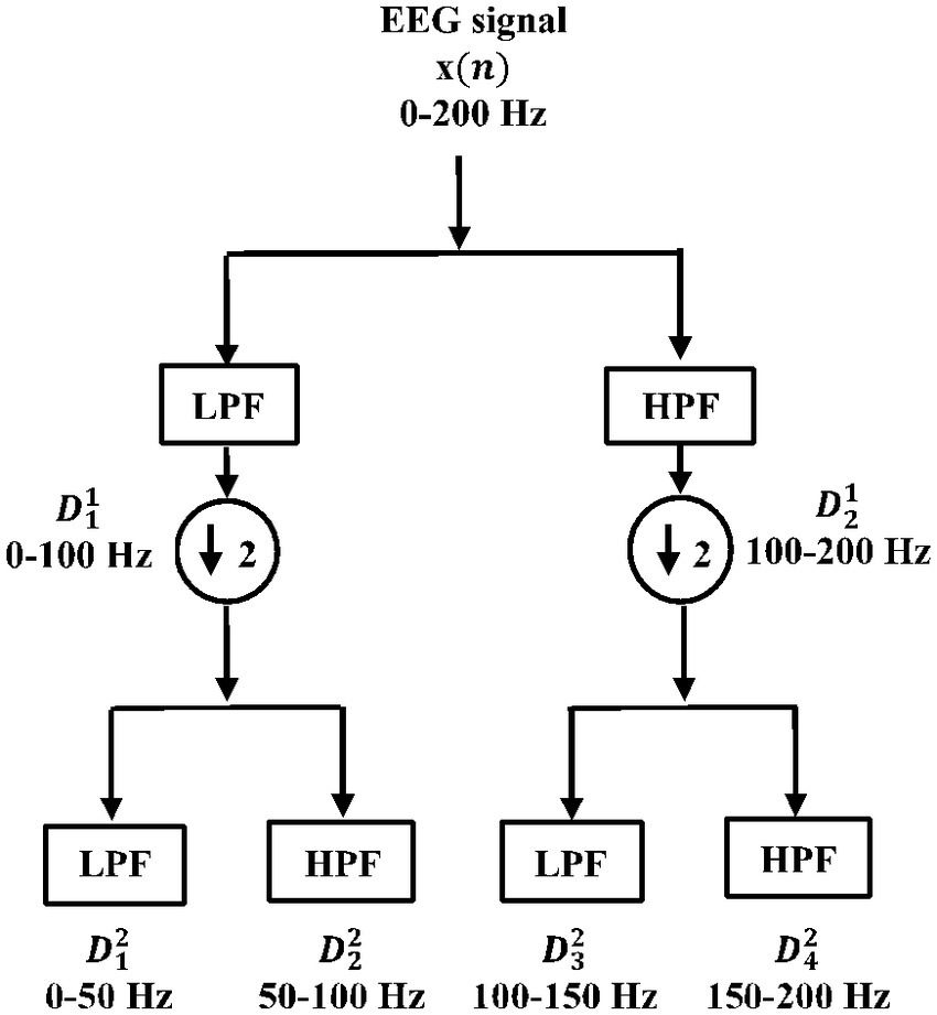
Figure 4. Double-branched architecture of wavelet packet transform (WPT).

2.2.2 Features derived from phase space representations (PSRs)

The visualization of phase space representations (PSRs) is useful for studying the dynamics and state of biomedical signals such as EEG (Sharma and Pachori, 2015; Swami et al., 2015b,c; Anuragi et al., 2022). The 3D PSRs are calculated by using equation (1).

PhaseSpaceRepresentationsPSRm=VmVm+τ…Vm+2τ    (1)

where, V represents EEG vectors of signal xn , τ represents the time lag, m=1,2,…,M−2τ , with total number of data points M . EEG signals are from elliptical paths, which are more irregularly shaped for ictal patterns (Swami et al., 2016b). The irregularities in the elliptical paths were quantified by evaluating Euclidean distances between the delayed vectors using equation (2).

EuclideandistancesEDm=Vm2+Vm+12+Vm+22    (2)

To highlight the differences between the Euclidean distances of the non-ictal versus ictal patterns in EEG signals, statistical features such as standard deviation SDpq or F1 (given by equation 3) and range (i.e., the difference between the maximum and minimum values) RNpq or F2 were calculated. Here, p is the number of segmented EEG signals and q is the number of wavelet coefficients (fixed to 128).

StandarddeviationvaluesSDpq=1Q−1∑q=1Qωpq−μpq2    (3)

The SDpq and RNpq are computed from all the 128 coefficients and considered as features for classification tasks.

2.2.3 Singular value decomposition (SVD) features or F3

The singular value decomposition (SVD) is a tool for decomposing a matrix into its Eigenvalues, which is suitable for a non-square matrix. Hence, it is a useful measure for extracting the algebraic properties from large data such as EEG to study its dynamics. The SVD covariance matrix C is given by equation (4).

Where singular values S=diagσ1,σ2,σ3,…,σN,0,…0 consists of a diagonal matrix with singular values σ1,σ2,σ3,…,σN , while, U=u1,u2,u3,…,ui∈Ri×i and V=v1,v2,v3,…,vj∈Rj×j represent unitary matrices. The singular values were calculated for each coefficient of the last decomposition level, and the final matrix is denoted by SVDpq . Hence, 128 singular values are considered for classification.

2.2.4 Energy features or F4

The abrupt neuronal discharges during the episodes of epileptic seizures consume high energy levels of the brain. This creates a misbalance between the energy levels within the brain. Hence, the evaluation of energy (EN) features directly from the wavelet coefficients allows us to quantify the difference between the energy levels during non-ictal and ictal events (Swami et al., 2016a). In this study, EN features are computed from all 128 coefficients and denoted as ENpq .

Finally, the complete feature matrix was formed by the horizontal concatenation of all the 512 (128 coefficients × 4) features given by equation (5).

Fpq=SDpqRNpqSVDpqENpq=F1F2F3F4    (5)

Where p is the index for EEG segments, q is the index for features, and it equals 1, 2, 3, …, 512. For the selection of the optimum number of features, the entire feature matrix Fpq was provided as input to the evolutionary multi-objective optimization model.

2.3 Evolutionary multi-objective optimization (EMO) using non-dominated sorting genetic algorithm (NSGA)-II

The GA is an evolutionary computing algorithm that is based on biological evolution. In multi-objective GA, more than one objective is optimized simultaneously to achieve the best-compromised solution (Deb, 2001; Smith, 2002). In this study, we have used the NSGA-II method for minimization of the number of required features and the error rate simultaneously. The steps involved in NSGA-II for minimizing the required objective functions are as follows:

i. Initialized random population pop for Fpq .

ii. Evaluated objective functions Oi . The first objective function O1 considered in this study is the minimum number of features required for the classification of non-ictal and ictal patterns. This is set randomly.

iii. The second objective function O2 considered is the mean error rate Er after 10 iterations of randomized sub-sampling cross-validation. The calculation of Er and the randomized sub-sampling procedure are illustrated as follows:

a. Error rate Er : In this study, the Er corresponds to the classification error for the segregation of non-ictal and ictal patterns. It is given by Fawcett (2006).

Here, CA is the mean classification accuracy calculated using equation (7).

CA=TN+TP/FP+FN+TN+TP×100%    (7)

Where TP represents true positive values,

TN represents true negative values,

FP represents false positive values, and

FN represents false negative values.

a. Cross-validation by randomized sub-sampling: It is a statistical cross-validation procedure in which the original input data are randomly subdivided into training and testing sets. This process was iterated 10 times, and an equal number of training and testing sets were formed. During each iteration, the CA of the model was evaluated. Here, a generalized regression neural network (GRNN) (illustrated in the next section) was employed for classification. Finally, the mean CA (in %) was subtracted from 100 to evaluate the measure of mean Er (in %), which formed the second objective of this study.

i. Applied non-dominated sorting (NDS) to sort the pop . Each chromosome pop1,pop2,pop3,….popn in the population was assigned rank along with its crowding distance. The crowding distance is the Euclidean distance between each individual in the front based on objectives.

ii. Performed selection based on the crowded comparison operator <n .

iii. Generated offspring population popc using cross-over and mutation operations (Heris, 2015).

iv. Evaluated objective functions for popc . During this process, the offspring population popc are combined with the current pop .

v. The NDS was again applied and the selection of the individuals for the next iteration was performed based on rank and the crowding distance assigned.

vi. The next iteration is filled subsequently by each Pareto front. If by adding all the elements from a Pareto front, population size exceeds p (i.e., number of signals), then individuals from that Pareto front are taken based on crowding distance in descending order till population size reaches p .

vii. Steps iv–ix are repeated until the algorithm converges.

viii. Once the algorithm converges, the Pareto front is made based on the chromosome’s rank and crowding distance. The solution is achieved based on tournament selection.

The rank 1 Pareto front of the University of Bonn (UoB) datasets is depicted in Figures 5, 6. Figure 5 resulted from subjecting the NSGA-II method to 500 iterations with a population size of 10, while Figure 6 was generated using the same method but with a population size of 20. The selected solution after step xi is highlighted in both Figures 5, 6. Similarly, the results of the rank 1 Pareto front for the Neurology & Sleep Centre (NSC) datasets are presented in Figures 7, 8. Additionally, the results for the Sri Ganga Ram Hospital (SGRH) datasets are shown in Figures 9, 10. Figures 7, 9 were obtained when the NSGA-II method underwent 500 iterations with a population size of 10, whereas Figures 8, 10 were generated with a population size of 20 under the same method.

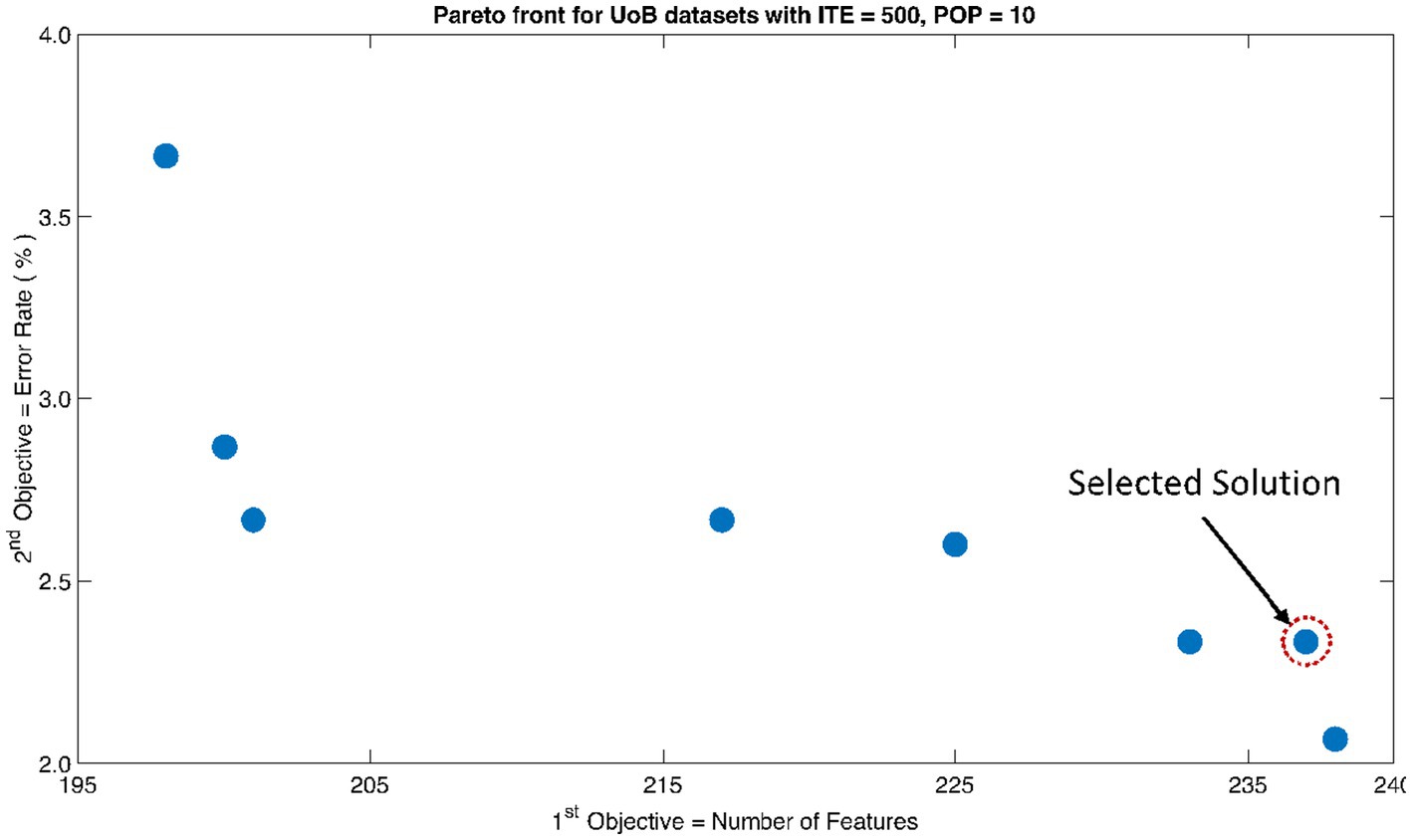
Figure 5. Non-dominant Solutions for University of Bonn (UoB) datasets when subjected to 500 iterations (ITE) and 10 population size (POP).

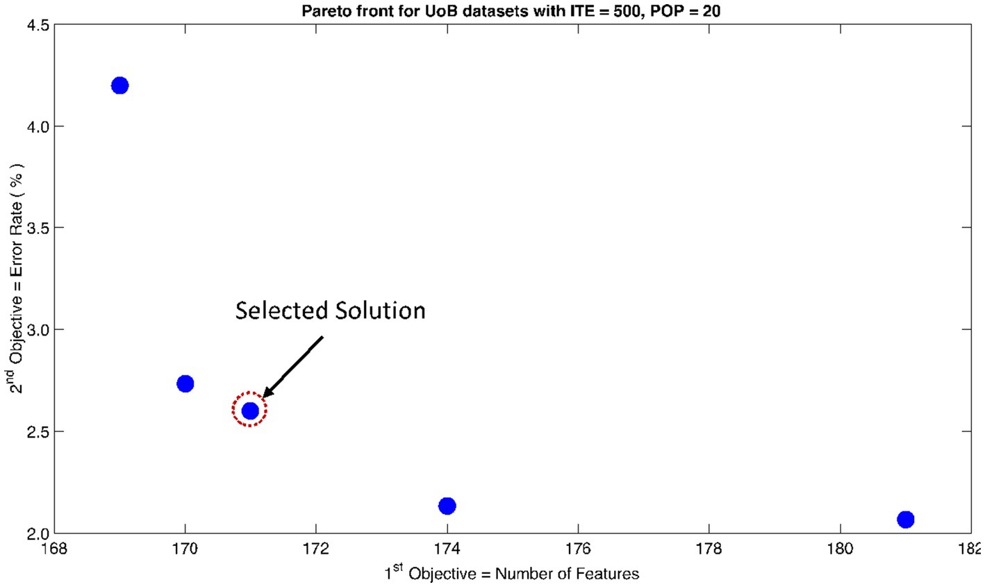
Figure 6. Non-dominant Solutions for University of Bonn (UoB) datasets when subjected to 500 iterations (ITE) and 20 population size (POP).

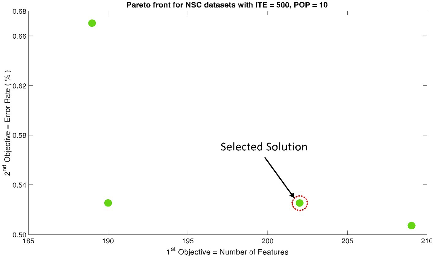
Figure 7. Non-dominant Solutions for Neurology & Sleep Centre (NSC) datasets when subjected to 500 iterations (ITE) and 10 population size (POP).

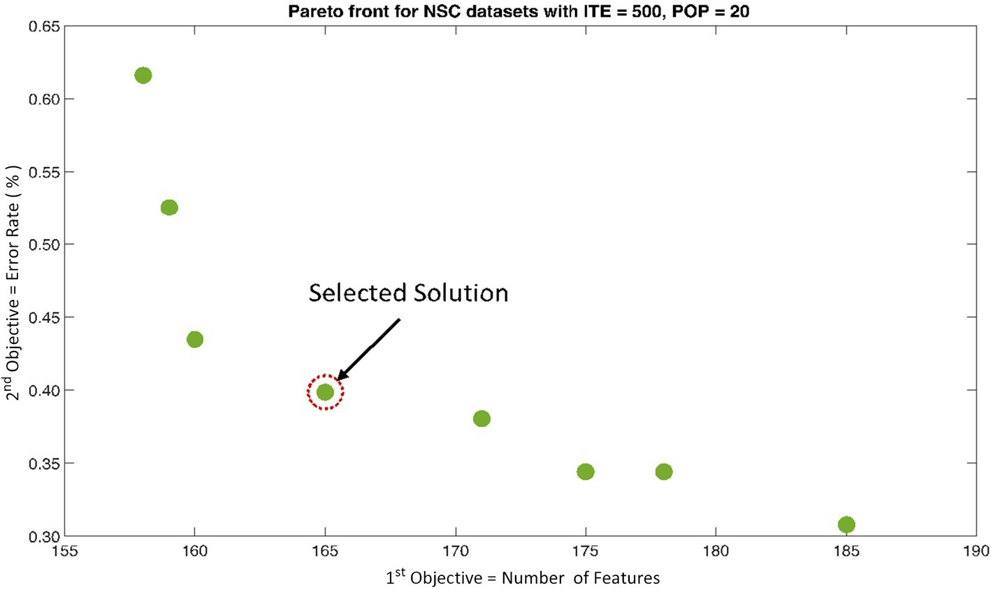
Figure 8. Non-dominant Solutions for Neurology & Sleep Centre (NSC) datasets when subjected to 500 iterations (ITE) and 20 population size (POP).

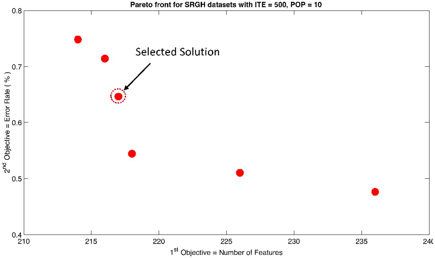
Figure 9. Non-dominant Solutions for Sri Ganga Ram Hospital (SRGH) datasets when subjected to 500 iterations (ITE) and 10 population size (POP).

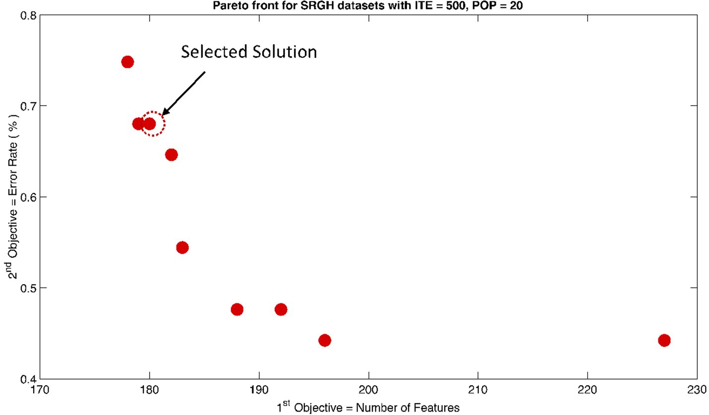
Figure 10. Non-dominant Solutions for Sri Ganga Ram Hospital (SRGH) datasets when subjected to 500 iterations (ITE) and 20 population size (POP).

2.4 Generalized regression neural network (GRNN) based classification

In artificial intelligence (AI), the classifier usually maps the function of input feature space to output class space. This could be mathematically expressed as f:Ra→Rb , where f represents the function, a is the dimension of input feature space, and b is the dimension of output feature. In neural networks, this mapping is achieved by the simulation of artificial neural clusters, such as the human brain. The GRNN model predicts the output/target class by predicting the probability density functions of the input data. GRNN has a memory-based architecture, and the solution is converged to the regression surface by following an asymptotic curve (Specht, 1991; Tomand and Schober, 2001). The parallel and one-pass learning architecture of the GRNN model is a lot faster than the recurrent neural networks.

The typical architecture of GRNN could be divided into four layers (shown in Figure 11). The input layer is the first layer of the GRNN model, which distributes the input data X among all the neurons after scaling. The second layer is the pattern or hidden layer. It applies the radial basis function to the probability density estimates. The spread of the radial basis function follows a Gaussian-shaped curve and is directly dependent on the value of the smoothing parameter σ . The measured values are passed into the next layer’s neurons, which consists of the summation units (one in the denominator and the other in the numerator). The denominator unit sums input weights dwj for all the samples from the pattern layer’s neurons. Similarly, the numerator unit sums the weights nwj for all the samples with actual targets of the pattern layer’s neurons. The final values of the numerator and the denominator have been indicated by ε1 and ε2 , respectively. The final layer of the GRNN model acts like an accumulator, which divides the ε1 and ε2 inputs to predict the output value ẐX . This value could also be expressed by assuming function fXY as the probability density of random variables X and Y . The density estimation is f̂XY for samples Χi and Yi, where i is the indices of the samples. The final predicted targets ŶΧ for p number of signals is given by equation (8).

ŶX=∑i=1pYie−δi22σ2/∑i=1pe−δi22σ2    (8)

Where scaling function δi2=Χ−ΧiTΧ−Χi.

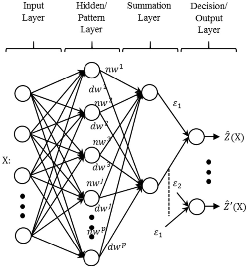
Figure 11. Typical architecture of generalized regression neural network (GRNN).

Based on equation (6), the outputs are similarly updated for Ŷ′Χ values.

Performance parameters: The following parameters were considered for evaluating the performance of the expert system developed:

Classification Accuracy (CA): It is the measure of the expert system to correctly classify the signals in the testing set as given by equation (7).

Sensitivity (SN): It is the statistical measure of the expert system to correctly classify the ictal patterns in EEG. It is evaluated by equation (9).

SN=TPFN+TP×100%    (9)

Specificity (SP): It is the statistical measure of the expert system to correctly classify the non-ictal patterns in EEG. It is evaluated by equation (10).

SP=TNFP+TN×100%    (10)

Mathew’s Correlation Coefficient (MCC): It is a balanced statistical measure that considers both the sensitivity and specificity values of the expert system. It is calculated using equation (11) (Jurman et al., 2012). The value varies from -1 to 1. The closer the value of MCC toward 1, the better the prediction (Jurman et al., 2012).

MCC=TP×TN−FP×FNTP+FPTP+FNTN+FPTN+FN    (11)

Computation Time (CT): It is the measure of the total time elapsed for classifying the signals in the testing set. In this study, CT was measured in s.

3 Results and discussion

In this study, datasets from three different repositories were evaluated for the classification of interictal (non-ictal) versus ictal patterns. Each dataset was decomposed into WPT coefficients, and various types of features were extracted, resulting in a total of 512 features. These features underwent EMO using the NSGA-II method. The unoptimized and optimized feature sets were then inputted into the GRNN ML classifier. Performance parameters, including CA, SN, SP, MCC, and CT, were extracted. Subsequently, a one-way analysis of variance (ANOVA) was conducted across the results of each dataset.

In each of Tables 1–3, OF1 represents the optimum features selected for the specific dataset when NSGA-II was subjected to 500 iterations and a population size of 10. Similarly, OF2 denotes the optimum features selected for the specific dataset when NSGA-II was subjected to 500 iterations and a population size of 20.

Table 1. Classification results using University of Bonn (UoB) datasets.