Overview

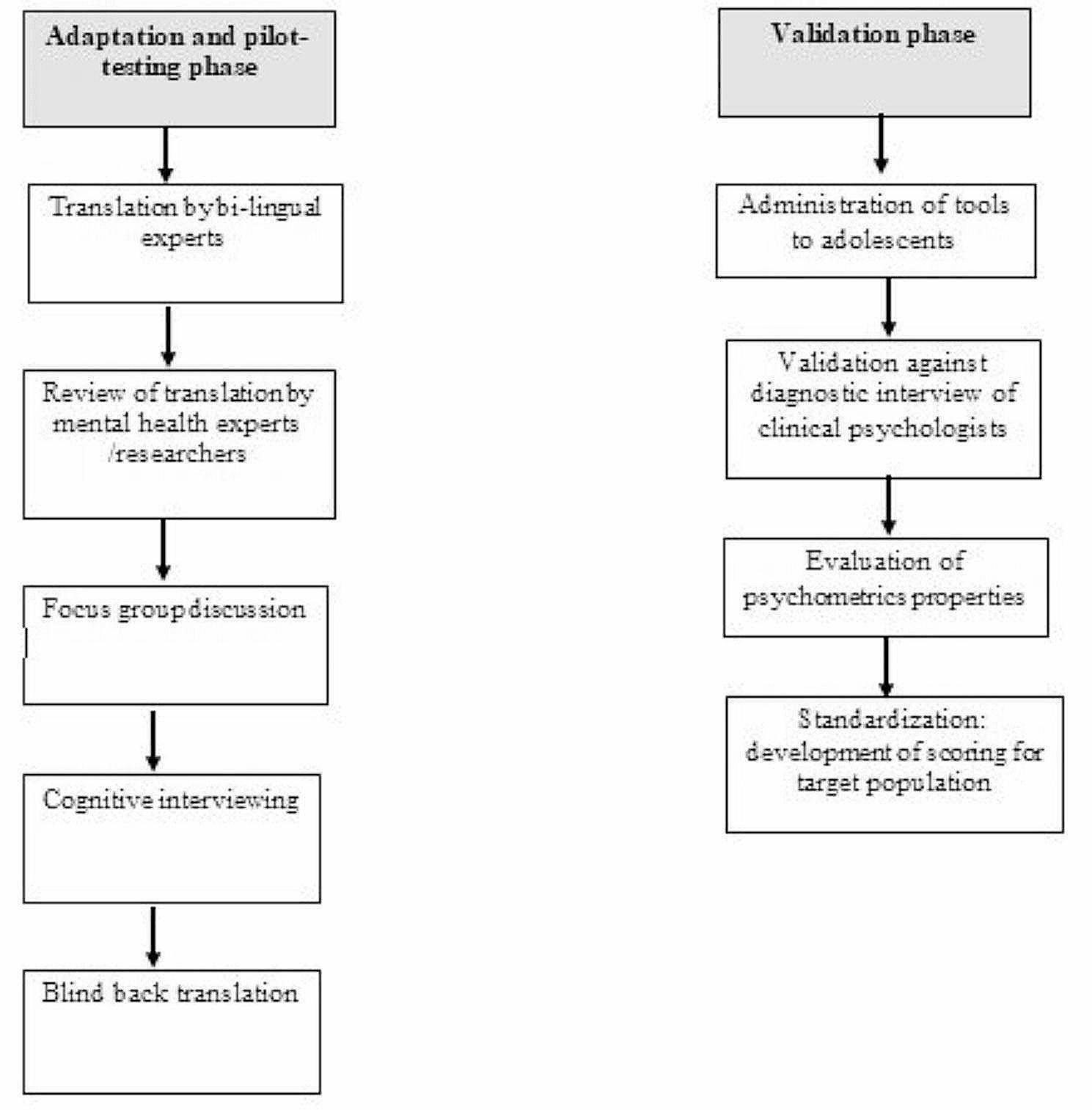
Our method included two phases, i.e., movement detection and characterization and feature discriminability analysis, as shown in Fig. 1. In the phase of movement detection and characterization, skeleton detection was performed by the “openpose” on each subject’s outpatient video to detect the corresponding skeleton sequence. Then, the corresponding set of 11 skeleton parameter sequences was calculated from each subject’s detected skeleton sequence. After that, the average variance of each of 11 skeleton parameter sequences was calculated by a sliding window approach, resulting in an 11-dimensional feature vector. Finally, the dataset of all subjects’ feature vectors and corresponding labels was obtained. In the next phases, i.e., feature discriminability analysis, the statistical comparison, cutoff, and classification were performed on the obtained dataset to verify the discriminability of each feature and each feature combination. For each feature, the statistical comparison analysis was applied to present the statistical significance between ADHD and non-ADHD; the cutoff analysis was used to find the optimal cutpoint and calculate the corresponding performance indices. To further discover the discriminability of multiple features, the classification analysis based on 17 feature combinations and six well-known machine learning classifiers was performed, and the corresponding performance indices and ranking were calculated.

Fig. 1

Flowchart of the proposed approach

Participants

We included 48 children (26 males and 22 females, mean age: 7 years 6 months ± 2 years 2 month) with ADHD (ADHD group) and 48 children (26 males and 22 females, mean age: 7 years 8 month ± 2 years 2 months) without ADHD (non-ADHD group), all of whom were examined by a pediatric neurologist and asked to sit on a chair for data recording. A diagnosis of ADHD was made in accordance with DSM-V criteria. ADHD severity was evaluated using the 26-item Swanson, Nolan, and Pelham Rating Scale (SNAP-IV), including 18 items on ADHD symptoms (nine related to inattentiveness and nine related to hyperactivity/impulsiveness) and eight items on oppositional defiant disorder symptoms specified in DSM, Fourth Edition criteria. Each item measures the frequency of the appearance of symptoms or behaviors, in which the observer indicates whether the behavior occurs “not at all”, “just a little”, “quite a bit”, or “very much”. The items were scored by observer on a 4-point scale from 0 (not at all) to 3 (very much). The ADHD is divided into three major type: inattentiveness (ADHD-I, children with this type of ADHD exhibit no or few signs of hyperactivity or impulsivity. Instead, the children will get distracted easily and difficult to pay attention), hyperactivity/impulsivity (ADHD-H, the children will demonstrate signs of hyperactivity and the need to move constantly and display impulsive behavior. They show no or few signs of getting distracted or inattention), and combined (ADHD-C, the children will demonstrate impulsive and hyperactive behavior and get distracted easily). To prevent biased comparison, children with a history of intellectual disability, drug abuse, head injury, or psychotic disorders were excluded from the ADHD group. The diagnoses in the patients without ADHD were headache, epilepsy, and dizziness, which are common in pediatric neurology. Written informed consent was obtained by a participant’s family member or legal guardian after the procedure had been explained. In addition, informed consent was also obtained from them for the publication of their children’s images. This study was approved by the Institutional Review Board of Kaohsiung Medical University Hospital (KMUIRB-SV(I)- 20190060).

Movement detection and characterization

We propose an objective and automatic approach to evaluate the movements of patients with ADHD and compare them with those of patients without ADHD. This approach is mainly based on movement quantization through the analysis of variance in patients’ skeletons detected automatically in outpatient videos (specifically, 4–6-min video recordings per patient). The 2D camera (I-Family IF-005D) was used to capture movement videos of each patient, with video recordings obtained at a frame rate of 30 Hz for each patient and a resolution of 1280 × 720. The camera was placed in a fixed position in the consulting room, as shown in Fig. 2. To minimize comparison bias, only the initial 4-min video recording was considered for analysis. To quantify the patients’ movements in an outpatient video objectively and automatically, we used OpenPose for detecting the patient’s skeleton in each video frame. This study employed two-dimensional (2D) real-time multiperson skeleton detection [12]. Figure 3 presents an example of the detected skeleton of a patient represented by 25 key points (joints): nose (0), neck (1), right shoulder (2), right elbow (3), right wrist (4), left shoulder (5), left elbow (6), left wrist (7), middle hip (8), right hip (9), right knee (10), right ankle (11), left hip (12), left knee (13), left ankle (14), right eye (15), left eye (16), right ear (17), left ear (18), left big toe (19), left small toe (20), left heel (21), right big toe (22), right small toe (23), and right heel (24). The detection result of each skeleton was represented by the 2D coordinates of these 25 joints in the image domain.

Fig. 2

The camera’s position and view in the consultation room

Fig. 3

Example of a patient’s skeleton detection. A detected patient’s skeleton represented by 25 key points and the corresponding skeleton parameters: a detected skeletons; b 25 key points; c shoulder-related and hip-related parameters; and d) thigh-related and trunk-related parameters

Assume \( P^ = \$}} _ ^|i = }, \ldots,24\} \) is the set of the 25 detected joints in the \(t\)th frame of an outpatient video. Let the frame coordinate of the \(i\)th joint \($}}}}_}^\) be represented by \((_}^,_}^)\), where \(_}^\in \,\dots,_-1\}\) and \(_}^\in \,\dots,_-1\}\). \(_\) and \(_\) are the frame’s width and height, respectively. On the basis of the natural connections (bones) between some pairs of joints, several bone vectors were defined, such as the right shoulder \($}}} }_}^=(_}^-_}^,_}^-_}^)\) from the neck joint \( \overset$}}}_}^\) to the right shoulder \($}}} }_}^\) and the left shoulder \($}}} }_}}^=(_}^-_}^,_}^-_}^)\) from the neck joint \($}}} }_}^\) to the left shoulder \($}}} }_}^\). To extract the skeleton’s features for characterizing patients’ movements and differentiate them between the ADHD and non-ADHD groups in outpatient videos, two types of skeleton parameters were defined, namely bone length and bone angle. For a bone vector \($}}} }_}^=(_}^-_}^,_}^-_}^)\), bone length \(_^\) was defined as follows:

$$_^=\sqrt[2]_}^-_}^\right)}^+_}^-_}^\right)}^},$$

(1)

Bone angle \(_^\) was defined as follows:

$$_^=\left|}^\left[\frac_}^-_}^\right)}_}^-_}^\right)}\right]\times \frac\right|.$$

(2)

On the basis of the patients’ movements observed in outpatient videos, six bone vectors, namely the right shoulder, left shoulder, right hip, left hip, right thigh, and trunk, were selected, and the corresponding lengths and angles were calculated. In addition to the right shoulder and left shoulder defined previously, four bone vectors were defined as follows:

1.

Right hip \($}}} }_}}^=(_}^-_}^,_}^-_}^)\) from the middle hip joint \($}}}_}^\) to the right hip \($}}}_}^\);

2.

Left hip \($}}} }_}}^=(_}^-_}^,_}^-_}^)\) from the middle hip joint \($}}}_}^\) to the left hip \($}}}_}^\);

3.

Right thigh \($}}} }_}}^=(_}^-_}^,_}^-_}^)\) from the right hip joint \($}}}_}^\) to the right knee joint \($}}}_}^\);

4.

Trunk \($}}} }_}}^=(_}^-_}^,_}^-_}^)\) from the neck joint \($}}}_}^\) to the middle hip joint \($}}}_}^\).

The right thigh was selected instead of the left thigh because the left thigh was usually partially occluded by the right thigh owing to the seated position of the patient. The corresponding lengths and angles of all bone vectors except the trunk were calculated using Eqs. (1) and (2), respectively, resulting in five length-related skeleton parameters, namely \(_^\), \(_}^\), \(_}^\), \(_}^\), and \(_}^\), and five angle-related skeleton parameters, namely \(_^\), \(_}^\), \(_}^\), \(_}^\), and \(_}^\). The corresponding angle of trunk bone vector \(_}^\) was calculated using the following equation:

$$_}^=\left\_^,& if\,\, _^\ge 0\\ _^+180,& if \,\,_^<0\end\right. } \,\,_^=}^\left[\frac_}^-_}^\right)}_}^-_}^\right)}\right]\times \frac.$$

(3)

Eleven skeleton parameters were extracted to characterize the detected skeleton in each frame of an outpatient video. For an outpatient video composed of \(T\) frames, \(T\) detected skeletons were present. The corresponding \(T\) values of each skeleton parameter constituted a time series. Thus, 11 time series corresponding to 11 skeleton parameters were obtained to characterize the detected skeleton sequence in the video.

Let \(}_^=(_^,_^,\dots,_^)\) and \(}_^=(_^,_^,\dots,_^)\) be the two series of the length and angle, respectively, corresponding to bone vector \($}}}_}^\). To characterize the variation in values in each series, the averaged variances of series \(}_^\) and \(}_^\) were calculated using a sliding window approach:

$$^\left(}_^\right)=\frac\sum _^^\left(\varvec}_^\right), ^\left(\varvec}_^\right)=\frac\sum _^_^-m\left(}}_^\right)\right)}^$$

(4)

$$^\left(}_^\right)=\frac\sum _^^\left(\varvec}_^\right), ^\left(\varvec}_^\right)=\frac\sum _^_^-m\left(\varvec}_^\right)\right)}^$$

(5)

where \(}}_^=\left(_^,_^,\dots, _^\right)\) and \(}}_^=\left(_^,_^, \right.\)\(\left.\dots,_^\right)\), \(r=\left(k-1\right)\times R+1\), are the \(k\)th subsequences of \(}_^\) and \(}_^\) with a window size of \(R\); \(m\big(}}_^\big)\) and \(m\big(}}_^\big)\) are the corresponding means; \(^\big(}}_^\big)\) and \(^\big(}}_^\big)\) are the corresponding variances; and \(K\) is the number of subsequences. Thus, 11 values of feature descriptors, \(^\left(}_^\right),\) \(^\left(}_}^\right),\) \(^\left(}_}^\right),\) \(^\left(}_}^\right),\) \(^\left(}_}^\right),\) \(^\left(}_^\right),\) \(^\left(}_}^\right),\) \(^\left(}_}^\right),\) \(^\left(}_}^\right),\) \(^\left(}_}^\right),\) and \(^\left(}_}^\right)\), were obtained to characterize the patient’s movement in an outpatient video. Finally, a two-dimensional dataset matrix with \(96\) rows and 12 columns was obtained for the following feature discriminability analysis. Note that each row corresponds to one subject’s 11 feature descriptor values (i.e., 11 averaged variances of skeleton parameters’ series detected from the initial 4-minute video recording) and one class label (ADHD or non-ADHD).

Feature discriminability analysis

To evaluate and compare the discriminating power of different features between the ADHD and non-ADHD groups, we determined an optimal cutoff. We adopted bootstrapping to prevent highly variable results and systematic overestimation of the out-of-sample performance. Let \(S=\left\_,_\left)\right|n=1,2,\dots,96\}\) be the original sample set of the feature descriptor to be evaluated, where \(_\) and \(_\) are the corresponding value and class label, respectively, of the nth patient. Each time, a so-called “bootstrap” or in-bag sample set \( \tilde \), with the same size (i.e., 96) as that of \(S\), was drawn randomly with replacement, and samples not drawn constituted a so-called “out-of-bag sample set.” On average, an in-bag sample set \( \tilde \) included 63.2% of all the samples of original sample set \(S\) because some samples were drawn multiple times [19]. An optimal cutpoint was determined by computing the performance index of discriminative ability at each value of the feature descriptor in the in-bag sample set \( \tilde \), and then selecting the feature value with the largest Youden index (defined as \(sensitivity+ specificity-1\)) value as the optimal cutpoint. Note that \(Sensitivity\) was the percentage of the correct prediction of the class “ADHD” for all patients in the ADHD group, while \(Specificity\) was the percentage of the correct prediction of the class “non-ADHD” for all patients in the non-ADHD group. After that, the obtained optimal cutpoint was applied to the out-of-bag sample set, and the corresponding four performance indices, namely \(accuracy\), \(sensitivity\), \(specificity\), and area under the receiver operating characteristic curve \((AUC)\), were calculated. \(Accuracy\) was the percentage of the correct prediction of the “ADHD” or “non-ADHD” class for all patients in both the groups. \(AUC\) was plotted with pairs of values of \(1- specificity\) and \(sensitivity\) corresponding to binary classification results obtained using different classification threshold values. The above process of optimal cutpoint searching in an in-bag sample set and testing in the corresponding out-of-bag sample set was repeated 100 times and the 100 different optimal cutoff values each with the corresponding values of four test performance indices were obtained. Finally, the average optimal cutpoint and four average test performance indices were calculated for evaluating the feature descriptor’s discriminating power between the ADHD and non-ADHD groups based on the cutoff analysis.

To evaluate the discriminating power of different feature combinations between the ADHD and non-ADHD groups, we performed classification analysis based on six machine learning classifiers and employed hyperparameter tuning with five-fold cross-validation to identify the most suitable model parameters. The adaptive boosting (AdaBoost) model’s weak classifiers were implemented with the classification and regression tree (CART) algorithm, and the corresponding parameter n-estimators were optimized within . The decision tree classifiers were implemented with CART algorithm, and the corresponding parameter max-depth was optimized within . The k-nearest neighbors (KNN) model’s parameter n-neighbors was optimized within . The random forest model’s parameters max-features, max-depth, and n-estimators were optimized with a grid search within , , and , respectively. The support vector machine (SVM) model’s kernel type was set as the radial basis function, and the corresponding parameters gamma and C were optimized with a grid search within and , respectively. The extreme gradient boosting (XGBoost) model’s weak classifiers were implemented with the CART algorithm, and the corresponding parameters learning rate, max-depth and n-estimators were optimized with a grid search within , , and , respectively. Seventeen feature combinations were evaluated and compared, including the 11 single features and six additional feature combinations—two thigh-related features (thigh-related) \(\^\left(}_}^\right),^\left(}_}^\right)\},\) four shoulder-related features (shoulder-related) \(\^\left(}_^\right), ^\left(}_}^\right), ^\left(}_^\right),^\left(}_}^\right)\},\) four hip-related features (hip-related) \(\^\left(}_}^\right),^\left(}_}^\right), \)\(\^\left(}_}^\right), ^\left(}_}^\right)\},\) five length-related features (length-related) \(\^\left(}_^\right), ^\left(}_}^\right), ^\left(}_}^\right),\)\(^\left(}_}^\right)\},^\left(}_}^\right),\) six angle-related features (angle-related)\(\^\left(}_}^\right), ^\left(}_^\right), ^\left(}_}^\right), ^\left(}_}^\right), \)\( ^\left(}_}^\right),\) \(^\left(}_}^\right)\},\) and all 11 features (all).

For each feature combination, the corresponding dataset comprised 48 feature vectors with “ADHD” labels and 48 with “non-ADHD” labels. To minimize the bias of model evaluation, the resampling strategy of 10-fold cross-validation was repeated 10 times. In each repetition, the dataset was equally and randomly partitioned into 10 folds, with each being composed of four to five “ADHD” and four to five “non-ADHD” feature vectors. Next, a fold was selected as the test dataset, and the remaining folds were selected as the training dataset. This training–test partitioning process was repeated 10 times, with each of the 10 folds being used only once as the test dataset. Moreover, the resampling strategies of 8:2 and 6:4 training-test random splits (holdout methods) with 100 repeats were also be applied for comparison. A total of 100 pairs of training and test datasets were obtained in each resampling strategy. For each pair, the training dataset was used to train the considered classifier and the test dataset was used to evaluate the trained classifier’s classification performance on the basis of four classification performance indices, namely accuracy, sensitivity, specificity, and AUC. The 100 values of each index corresponding to the 100 test datasets were averaged to estimate the classification test performance of the classifier. The larger the values of all four indices were, the stronger the discriminating power of the combination of the feature set and classifier was. To compare the discriminating power of the 17 feature sets across the six classifiers, the averaged ranking of each feature set corresponding to each classification performance index was calculated by averaging the feature set’s ranks in the corresponding index’s results of six classifiers. The smaller the averaged rank values of all four indices were, the stronger the discriminating power of the feature set was.

Statistical analysis

All statistical analyses were conducted using SAS (v9.3; SAS Institute, Cary, NC, USA). Data are presented as means ± standard deviation. Measurements between patients with and without ADHD were conducted using the two-sample t test. P < 0.05 was considered statistically significant.