Introduction

Brain areas are composed of highly heterogenous cell populations with diverse structure and function. An extensive knowledge about individual cell types is required to better understand the functional organization of neural systems at different levels. Over the past two decades, next-generation RNA sequencing (RNA-seq) has paved new roads to investigate the molecular determinants of cellular diversity (Macaulay and Voet, 2014; Svensson et al., 2018). In the present study, we took advantage of recent advances in RNA-seq technologies and employed patch-seq, a powerful multi-modal single-cell approach, to decipher the biophysical and transcriptomic determinants of neuronal heterogeneity in the lateral superior olive (LSO). The LSO is a conspicuous brainstem nucleus receiving and analyzing binaural input. It contains neurons in the ascending and the descending pathway, namely principal neurons (pLSOs) and lateral olivocochlear neurons (LOCs). pLSOs are involved in sound localization, whereas LOCs enable the central auditory system (CAS) to directly control the cochlear periphery (reviews: Friauf et al., 2019; Yin et al., 2019; Owrutsky et al., 2021).

pLSOs amount to almost 34 of all LSO neurons (Helfert and Schwartz, 1986, 1987; Franken et al., 2018), whose number slightly exceeds 1,600 in mice (Hirtz et al., 2011). By performing a subtraction-like process of excitatory and inhibitory input signals from the ipsi- and contralateral ear, respectively, pLSOs detect interaural level differences (Tollin, 2003). The main inputs are in strict tonotopic register and are glutamatergic, respectively, glycinergic with modulatory GABAergic inputs (Fischer et al., 2019). Collectively, these inputs are tuned for fast and precise synaptic transmission, even during sustained high-frequency stimulation (Krächan et al., 2017; Müller et al., 2022). pLSOs in mice have fusiform somata with a surface area of ~130 μm2 (Williams et al., 2022). For juvenile mice, an input resistance (Rin) of 96 MΩ, a resting potential (Vrest) of −64 mV, and a membrane capacitance (Cm) of 11 pF have been reported (Sterenborg et al., 2010). Another study found 70 MΩ, −57 mV and 22 pF for mouse LSO neurons in general (Leao et al., 2006). A striking feature of pLSO neurons is a prominent inward current (Ih) which is mediated through hyperpolarization-activated and cyclic nucleotide-modulated (HCN) channels (Leao et al., 2006; Sterenborg et al., 2010).

Two subpopulations of pLSOs can be distinguished by their intrinsic firing pattern in vitro (rats: Barnes-Davies et al., 2004). In mice, the first subtype, termed single spiking (Sterenborg et al., 2010) or onset-burst pLSOs (Haragopal and Winters, 2023), fires 1–5 action potentials (APs) of short latency during prolonged depolarization. The second pLSO subtype fires throughout the duration of the stimulus and has been termed multiple firing (Sterenborg et al., 2010) or multi-spiking (Haragopal and Winters, 2023).

pLSO neurons send ipsilateral, glycinergic projections to the intermediate nucleus and the dorsal nucleus of the lateral lemniscus (INLL, DNLL) as well as the central nucleus of the inferior colliculus (CNIC) (Figure 1A; Friauf et al., 2019; Mellott et al., 2022). pLSOs also give rise to contralateral, mainly glutamatergic projections terminating in the DNLL and CNIC (Saint Marie et al., 1989; Saint Marie and Baker, 1990; Glendenning et al., 1992; Fredrich et al., 2009; Abraham et al., 2010). As recently reported, both projection types contribute relatively equally to the pLSO output in mice (Haragopal et al., 2023).

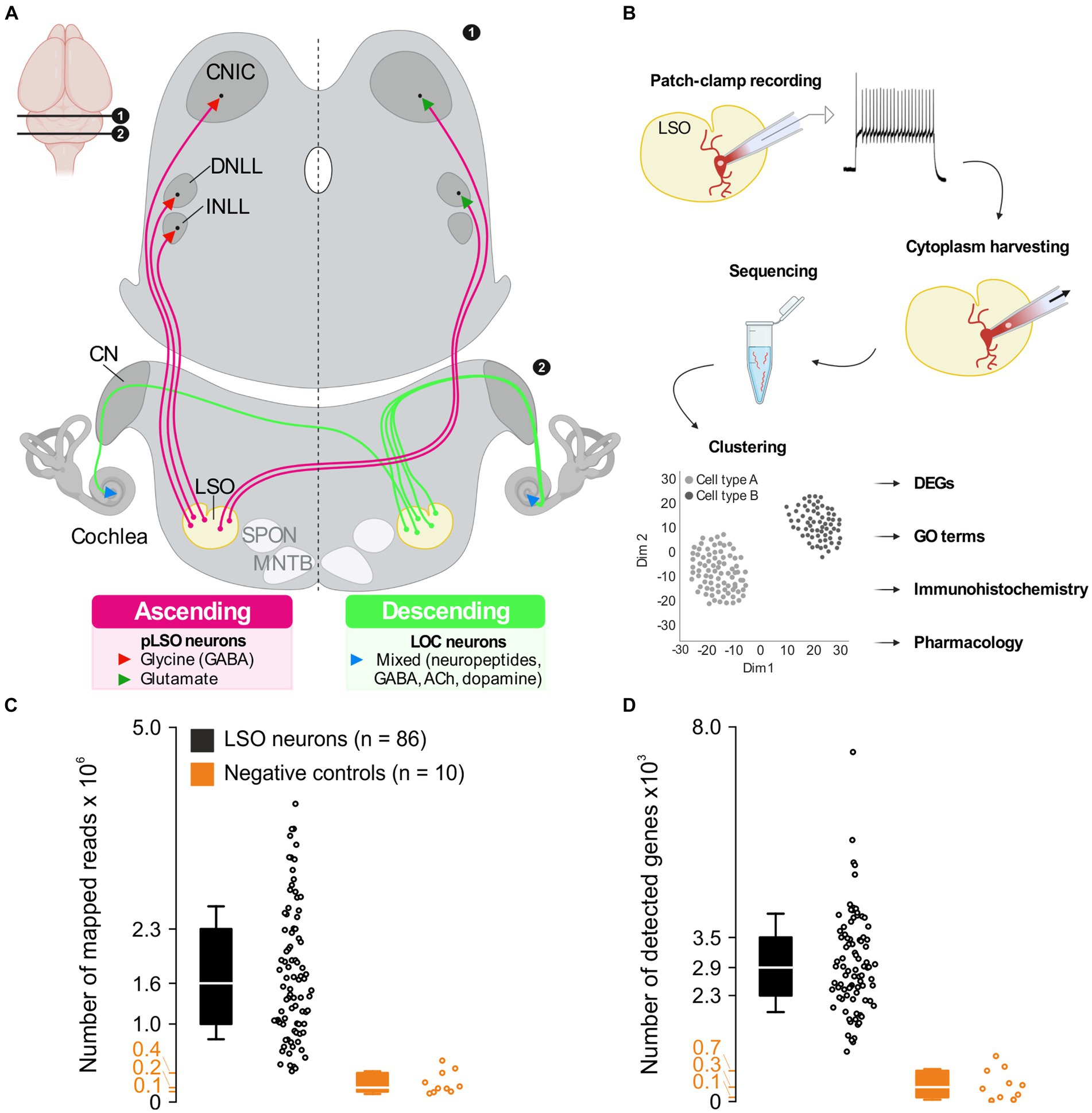
Figure 1. A priori quality checks result in 86 LSO patch-seq neurons of sufficient quality. (A) Ascending projections (left) and descending projections (right) of LSO neurons. Inset (top left) depicts position of coronal sections in the brain. (B) Patch-seq workflow. Whole-cell patch-clamp experiments were performed to assess electrophysiological properties, followed by cytoplasm harvesting. The cytoplasm was used for cDNA library synthesis and sequencing. After processing sequencing reads, unsupervised clustering was done to identify neuron types, and further analyses were performed to characterize these neuron types. (C) Number of mapped reads from 86 LSO neurons of sufficient quality and 10 neurons from negative controls (black and orange, respectively). (D) As (C), but for detected genes. CN, cochlear nuclear complex; CNIC, central nucleus of the inferior colliculus; DNLL, dorsal nucleus of the lateral lemniscus; INLL, intermediate nucleus of the lateral lemniscus; LSO, lateral superior olive; MNTB, medial nucleus of the trapezoid body; SPON, superior paraolivary nucleus. See also Supplementary Figures S1, S2. In these and all subsequent box plots, center line marks median (Q2), box limits mark first and third quartile (Q1 and Q3), and whiskers represent standard deviation (SD).

LOCs are the second major neuron type in the LSO. They form one of the two branches of efferent projections of the auditory system, the second branch being composed of medial olivocochlear neurons (MOCs, reviews: Brown, 2011; Guinan, 2011). Ontogenetically, LOCs and MOCs have a motoneuronal nature (Karis et al., 2001; Simmons, 2002). The efferent auditory system comprises ~470 neurons (mice), with LOCs exceeding MOCs by ~2-fold (Campbell and Henson, 1988). In mice, LOC somata are round and have a surface area of ~100 μm2 (Williams et al., 2022); (Suthakar and Ryugo, 2021, report ~140 μm2). Most LOC somata are intrinsic to the LSO and intermingled with pLSO somata (mice); few somata reside in a shell region surrounding the LSO (Wu et al., 2020; Williams et al., 2022).

Axons of LOCs are thin and unmyelinated (Brown, 2011). Virtually all (99%) project into the ipsilateral cochlea (Guinan, 2018). The axons make en passant synapses primarily on radial “dendrites” of type I auditory neurons, beneath the basal pole of inner hair cells (Warr et al., 1997; Simmons, 2002). A minority of LOCs contact inner hair cells directly (Liberman, 1990; Sobkowicz and Slapnick, 1994; Sobkowicz et al., 1997). Furthermore, LOCs may project to the ventral cochlear nucleus (Ryan et al., 1990) and have axon collaterals terminating in the LSO itself and slightly outside (Brown, 1993). In line with the unmyelinated nature of their axons, peripheral effects of LOC activity are slower than MOC effects and occur over minutes. LOCs likely modulate auditory nerve fiber activity in a reflex manner (Guinan, 2011) and protect the cochlea against noise-induced hearing loss (Darrow et al., 2007; Fuchs and Lauer, 2019).

Like pLSOs, LOCs receive excitatory and inhibitory inputs, yet with longer latencies and slower kinetics (review: Friauf et al., 2019). They differ from pLSOs in several biophysical properties. For instance, they display a regular firing pattern in response to depolarizing current pulses injected in vitro, whereby the first AP occurs with a substantial and variable delay (25–180 ms; Adam et al., 1999). In contrast to pLSOs, LOCs lack Ih currents, but they exhibit prominent low-threshold and rapidly activating and inactivating transient outward K+ currents. By counteracting depolarizing effects of excitatory synapses, these currents are key determinants of synaptic integration and repetitive AP activity (Rothman and Manis, 2003; Manis, 2008). In accordance with their relatively small somata (Williams et al., 2022), mouse LOCs have an exceptionally low Cm (6 pF) (Sterenborg et al., 2010). The authors also reported a very high Rin (~300 MΩ) and a relatively positive Vrest (−43 mV). Low Cm values in LOCs were also obtained by Fujino et al. (1997) and Leijon and Magnusson (2014) (mouse, 15 pF; rat, 40 pF).

The neurochemistry of LOCs is complex. They are predominantly cholinergic but also contain various other transmitters (reviews: Brown, 2011; Sewell, 2011). In mice, GABAergic markers have been described in all cochlear LOC fibers (Maison et al., 2003). A smaller, non-cholinergic fraction of LOCs is dopaminergic (Eybalin et al., 1993; Gil-Loyzaga, 1995; Safieddine et al., 1997; Darrow et al., 2006). Besides these classical transmitters, several neuromodulators have been described, including calcitonin-gene-related peptide (CGRP) (Kresse et al., 1995; Maison et al., 2003; Wu et al., 2018; summaries: Robertson and Mulders, 2000; Le Prell et al., 2021), urocortin (Vetter et al., 2002; Kaiser et al., 2011), and opioid peptides such as dynorphin (Le Prell et al., 2014) or enkephalins (Eybalin, 1993; Safieddine et al., 1997). A cholinergic LOC may co-contain CGRP and opioids, and various opioids can co-localize as well (Altschuler et al., 1988; Safieddine et al., 1997; Frank et al., 2023). Therefore, LOCs belong to the growing category of multi-transmitter neurons. Taken together, LOCs, despite being only a few, dynamically fine-tune auditory nerve activity via the release of excitatory and inhibitory transmitters (Groff and Liberman, 2003). The functions of LOCs in hearing, however, are virtually unknown (Romero and Trussell, 2022). They are much less explored than MOCs, and many issues are still under investigation (Kitcher et al., 2022). For example, direct evidence that LOCs respond to sound is still missing (Fuchs and Lauer, 2019).

Previous research has primarily focused on the electrophysiological properties and differentiation of neurons in the LSO. Some studies explored the molecular determinants influencing these electrophysiological properties but used now outdated techniques such as serial analysis of gene expression (SAGE) (Koehl et al., 2004; Nothwang et al., 2006) or microarrays (Ehmann et al., 2013; Xiao et al., 2013). These methods have not been able to achieve single cell resolution, which is critical in heterogeneous nuclei such as the LSO. Recently, Frank et al. (2023) presented transcriptomic single-cell transcriptomic results for LOC neurons but not for pLSO neurons. Here, we combined electrophysiology and transcriptomics using the patch-seq technique to assess functional and molecular diversity in individual LSO neurons of juvenile mice. We functionally characterized cell types in brain slices, harvested the cytoplasm and performed genome-wide expression profiling. Our goal was to identify molecular determinants of cellular heterogeneity and similarity in the LSO. We identified two clusters, pLSOs and LOCs. Differential expression was found for 353 genes, including known and novel cell type-specific markers. In particular, Kv channel subunits were intensively analyzed. Our comprehensive study identified complex molecular fingerprints at the single-cell level, paving the way for a variety of follow-up studies.

Methods Animals and ethical approval

Animal breeding and experiments were approved by the regional councils of the Land Rhineland-Palatinate according to the German Animal Protection Law (TSchG §4/3) and followed the guidelines for the welfare of laboratory animals. C57BL/6 J mice were bred in the animal facilities of the University of Kaiserslautern, and both sexes were analyzed at postnatal day (P) 11 ± 1, i.e., around hearing onset.

Brainstem slices preparation and electrophysiology

RNase-free solutions were prepared, and equipment was cleaned as described (Cadwell et al., 2017). Coronal brainstem slices were prepared (Hirtz et al., 2011) and in vitro electrophysiology was performed as described (Müller et al., 2019). Briefly, slices were perfused with ASCF (in mM: 125 NaCl, 2.5 KCl, 1 MgCl2, 1.25 NaH2PO4, 2 sodium pyruvate, 3 myo-inositol, 0.44 L-ascorbic acid, 25 NaHCO3, 10 D-glucose, 2 CaCl2; pH 7.4 when oxygenated with carbogen). Whole-cell patch-clamp recordings from LSO neurons were performed at 36.5 ± 1°C. Patch pipettes were filled with internal solution (in mM: 140 potassium gluconate, 10 HEPES, 5 EGTA, 1 MgCl2, 2 Na2ATP, 0.3 Na2GTP). The internal solution contained 0.8% RNase inhibitor (Invitrogen). The liquid junction potential was 15.4 mV and was corrected online.

Current clamp

Vrest values are an average over a 30-s period (sample frequency 5 kHz, otherwise 50 kHz). The initial phase of the hyperpolarizing response to a − 200-pA, 200-ms current pulse was fitted mono-exponentially (OriginPro 9.1, OriginLab) to determine the membrane time constant (τm). Current pulses with increasing amplitude (−200–1,000 pA, in 50-pA steps, 200 ms) were used to approximate rheobase, determine AP latency at rheobase, firing pattern (150 pA above rheobase) and voltage sag (at −200 pA). Triangular current pulses (rise to peak 1.5 ms, decay to baseline 3.5 ms, 10 repeats) were injected to determine AP amplitude, threshold, halfwidth, and peak latency. AP halfwidth was measured at 50% of the AP peak amplitude from baseline.

Voltage clamp

A 200-ms negative voltage step from the holding potential (Vhold; −70 mV) to −75 mV was applied to determine series resistance (Rs) and Rin (sampled at 20 kHz). Membrane currents were recorded for 1 min at Vhold. Peak amplitudes of spontaneous postsynaptic currents (sPSCs) and their kinetics (10–90% rise time, 100–37% decay time constant τdecay) were determined at Vhold and analyzed using Mini Analysis 6 (Synaptosoft). With a Cl-reversal potential of −112 mV, inhibitory sIPSCs were outward currents. Thus, they could be easily distinguished from excitatory sEPSCs which were inward currents. For each neuron, 100 sIPSCs and 100 sEPSCs were averaged. Data analysis was performed using custom-written IgorPro 6 and IgorPro 8 routines (WaveMetrics), and Clampfit 10 (Molecular Devices). Data visualization was performed using IgorPro, OriginPro 9.1, and CorelDRAW Graphics Suite 2019 (Corel Corporation).

Cytoplasm harvesting

Electrophysiological characterization was limited to ~10–15 min to minimize mRNA degradation. Total RNA was then extracted into the patch pipette by gently aspirating the neuronal cytoplasm. Shrinkage of the soma and entry of the nucleus into the pipette were visually monitored under DIC optics (Supplementary Figures S1A1–A3). After successful harvesting, atmospheric pressure was restored and the pipette was slowly removed from the soma (Supplementary Figure S1B). In case of contamination of the pipette by extracellular material, absence of a membrane patch at the tip of the pipette, or soma swelling, samples were discarded (Supplementary Figures S1C1,C2,D1,D2). The contents of the pipette were collected in a reaction tube containing 2 μL lysis buffer, 0.2% Triton-X, ERCC RNA Spike-In Mix (Invitrogen, 1:400,000 dilution) and RNase inhibitor. Samples were stored at −80°C and processed further en bloc (library preparation and sequencing). From a total of 263 patched neurons, 103 were retained for further analysis. Ultimately, 86 neurons passed the RNA quality control (see below). One negative control was collected per experimental day. A pipette filled with internal solution was moved so that its tip touched the slice. It was then withdrawn, and the contents of the pipette were processed as for harvested cells.

Library preparation and sequencing

Double-stranded cDNA was generated as described, with minor modifications (Picelli et al., 2013). Briefly, 1 μL of 10 mM dNTPs and 0.5 μL of Oligo-dT primer (Supplementary Table S1) were added to each sample, and samples were incubated at 72°C for 3 min and immediately placed on ice. Reverse transcription was performed using 0.5 μL SuperScript II RT (200 U/μL, Invitrogen) supplemented with 0.25 μL RNasin (40 U/μL, Promega), 2 μL Superscript II first-strand buffer (5x), 0.48 μL 100 mM DTT, 2 μL 5 M betaine, 0.12 μL 0.5 M MgCl2, 0.1 μL 100 μM template-switching oligonucleotide and 0.25 μL nuclease-free water. Incubation was performed at 42°C for 90 min, followed by 10 cycles at 50°C for 2 min and another incubation step at 42°C for 2 min. Enzyme inactivation was achieved by incubation at 70°C for 15 min. cDNA was pre-amplified by adding 12.5 μL KAPA HiFi HotStart ReadyMix PCR Kit (Roche), 0.25 μL IS PCR primer and 2.25 μL nuclease-free water with these thermocycling conditions: 98°C for 3 min, 18 cycles at 98°C for 20 s, 67°C for 15 s, 72°C for 6 min and final elongation at 72°C for 5 min. cDNA was purified using 0.8 X Ampure XP Beads (Beckman Coulter) and elution in 7 μL RNase free water. Quality control of randomly selected cells was assessed on an Agilent Bioanalyzer using the HS DNA Kit. On average, 450 pg. of cDNA was used as input for dual-indexed Nextera XT library preparation (Illumina). A total of 9 cycles of library amplification were performed according to the manufacturer’s recommendations. All individual single-cell libraries were pooled in equal amounts prior to purification of 100 μL pooled libraries with 1X Ampure XP Beads (Beckman Coulter) and final elution in 15 μL RNase-free water.

Library quality control and next generation sequencing

Prior to sequencing, the library pool was quantified using the Qubit dsDNA HS Assay Kit (Invitrogen), and the fragment size distribution was checked using the High Sensitivity DNA Kit (Agilent) on an Agilent 2100 Bioanalyzer. The library pool was additionally quantified with the PerfeCTa NGS Quantification Kit (Quanta Biosciences) and normalized for clustering on a cBot (Illumina). Libraries were sequenced on a HiSeq2500 (Illumina) using dual index reads with 88 bp read length.

Processing and analysis of single-cell RNA-seq data

Initial quality control of the raw data was performed using FastQC. Reads were trimmed using Trim Galore! (v0.4.2) to remove 3′ ends with base quality below 20 and adapter sequences. Reads were aligned to the mouse genome mm10 using STAR (Dobin et al., 2013, v2.5.2a) with a 2-pass mapping strategy per sample. PCR duplicates were detected using MarkDuplicate from the Picard tools (version 1.115). Reads aligned to mm10 were summarized to Gencode annotation vM2 (Harrow et al., 2012) using featureCounts (Liao et al., 2014, v1.5.0-p3) and counting primary alignments only (Li and Dewey, 2011, v1.3.1).

For quality control, filtering, and normalization of single-cell RNA-seq (scRNA-seq) data, we used the SingleCellExperiment R package (version 1.8.0, Amezquita et al., 2020) and the scran package (version 1.14.6; Lun et al., 2016) on Bioconductor. The deconvolution method was used to remove cell-specific library size biases, and size factors were calculated for each library using the ComputeSumFactors function. Of 103 aspirated cells, 17 (~16%) were discarded due to poor sequencing quality, leaving 86 neurons. Poor quality cells had >3 median absolute differences below the median for number of counts or number of transcripts. Genes with an average of at least one count in at least 5% of the neurons qualified for downstream analysis, resulting in 11,659 expressed genes. Transcripts per million (TPM) values were calculated by normalizing for gene length and sequencing depth (Zheng et al., 2020). The top 500 highly expressed genes were selected for Kyoto Encyclopedia of Genes and Genomes (KEGG) enrichment analysis using gene set enrichment analysis (GSEA) performed with DAVID 2021 (Huang et al., 2009; Sherman et al., 2022).

Clustering was performed using SC3 (Kiselev et al., 2017) and Seurat (Satija et al., 2015). Principal component analysis (PCA) was performed using the Seurat function RunPCA (Lun et al., 2016). Normalized log2-transformed highly variable gene (HVG) counts were used as input. t-Distributed Stochastic Neighbor Embedding (tSNE) (Kobak and Berens, 2019) plots were generated with RunTSNE.

DEGs were detected using the findMarkers function from the scran package, which uses a t-test by default. A gene was defined as a DEG if the normalized count showed a ≥ 2-fold upregulation (log2FC ≥ 1) and a false discovery rate (FDR) ≤ 0.05 (-log10FDR ≤ 1.3). DEGs were ranked by their Area Under the Receiver-Operating Characteristic curve (AUROC). DEGs were also selected for Gene Ontology (GO) enrichment analysis using GSEA performed with DAVID 2021. GO terms were condensed using REVIGO (Jiang and Conrath algorithm) (Supek et al., 2011). UpSet plots were generated using the UpSetR package (v.1.4.0) (Conway et al., 2017).

Super DEGs and cluster similarity

DEG analysis is a widely used method for assessing differences between samples. However, at least one pitfall is associated with very low expression levels. A gene may qualify as a DEG even if the average expression level in the two samples is very low (e.g., Scn4b|Navβ4, DEG#173 in pLSO, showed 1.5 vs. 0.0 TPM; Supplementary Figure S8A and Supplementary Table S6). To account for this caveat, we applied a more stringent approach and condensed the DEGs that showed an expression level of ≥10 TPM in ≥1 cluster. If the normalized counts differed ≥4-fold (log2FC ≥ 2), these DEGs were defined as “Super DEGs.” In addition, we used the same “≥10 TPM in ≥1 cluster” criterion to determine “Cluster similarity,” defined as ≤2-fold difference between clusters (log2FC ≤ 1). We further assessed Cluster similarity by using the overlapping index (OI), a means to quantify the similarity of datasets in terms of their distributions (cf. chapter” Super DEGs and Cluster similarity between pLSOs and LOCs”; OI = 0 → no overlap, OI = 1 → perfect overlap; Pastore and Calcagni, 2019).

To make the data sets more explorable, we have added the file in Supplementary Table S6. It lists the complex gene expression profiles for each neuron and allows the user to interactively change the selection criteria, such as the TPM threshold, and to assess how the changes affect the percentage of cells expressing a gene.

Data availability statement

The single-cell RNA sequencing data generated during this research project has been submitted to NCBI GEO and can be accessed using the accession number GSE241761.

Immunohistochemistry

Lethally anesthetized mice (7% chloral hydrate, 0.01 mL/g body weight or 10% ketamine, 220 μg/g body weight plus 2% xylazine, 24 μg/g body weight) were transcardially perfused with 100 mM phosphate-buffered saline (PBS, pH 7.4) at room temperature (RT), followed by ice-cold 4% paraformaldehyde (PFA) for 20 min. Brains were removed from the skull, postfixed for 2 h in 4% PFA (4°C) and stored in 30% sucrose-PBS at 4°C overnight. For Kv7.2, Kv7.3, and osteopontin, brain fixation was performed with Zamboni solution. 30-μm-thick brainstem slices were cut with a sliding microtome (HM 400 R, MICROM) and transferred to 15% sucrose-PBS, followed by three rinses in PBS (30 min, RT). Incubation and rinsing steps were performed free-floating unless otherwise noted. For Kvβ3, a heat-induced epitope retrieval protocol was used prior to antibody treatment. For this, slices were immersed in 10 mM sodium citrate buffer (pH 6.0) plus 0.05% Tween 20 (Roth) and heated at 95°C for 20–40 min. They were then returned to RT, followed by three rinses in PBS (5 min, RT).

Fluorescence labeling

Sections were incubated in blocking solution (0.3% Triton X-100, 10% goat serum [donkey serum for osteopontin], 3% BSA in KCl-free PBS) for 2 h at RT. Antibodies to osteopontin (1:250, goat, R&D Systems), vGLUT1 (1:500, guinea pig, Synaptic Systems), GlyT2 (1:250, mouse, Synaptic Systems), CGRP (1:500, guinea pig, Synaptic Systems), Kv7.2 (1:500, rabbit, Synaptic Systems), Kv7.3 (1:500, rabbit, Synaptic Systems), Kv11.3 (1:250, rabbit, Alomone) and Kvβ3 (1:200, rabbit, Biomol) were applied overnight at 4°C in carrier solution (0.3% Triton-X-100, 1% goat serum [donkey serum for osteopontin], 1% BSA in KCl-free PBS) solution followed by three rinses in PBS (30 min, RT). The sections were then incubated for 90 min in the dark with secondary antibodies (1,500, goat anti-guinea pig AlexaFluor 488, goat anti-rabbit AlexaFluor 568, Thermo Fisher Scientific; goat anti-rabbit AlexaFluor 488, Invitrogen; goat anti-mouse AlexaFluor 568, donkey anti-goat AlexaFluor 488, Molecular Probes; donkey anti-goat AlexaFluor 568, Invitrogen). After three PBS rinses (30 min, RT), sections were mounted on gelatin-coated slides and coverslipped with mounting medium containing 2.5% 1,4-diazabicyclo [2.2.2] octane (Sigma-Aldrich). Images were captured with a TCS SP5 X confocal microscope equipped with an HCX PL APO Lambda blue 63x oil objective (Leica Microsystems).

3,3′-diaminobenzidine labeling

To block endogenous peroxidase, sections were incubated for 30 min in 10% methanol, 3% H2O2 KCl-free PBS, rinsed in PBS (three times 10 min, RT), and transferred to blocking solution for 2 h at RT. Primary antibodies against CGRP or osteopontin were applied overnight at 4°C, followed by three rinses in PBS (30 min, RT). The sections were then incubated with biotinylated secondary antibodies (1:100, goat anti-guinea pig, Rockland; 1:100, donkey anti-goat, Jackson) in carrier solution for 90 min at RT and rinsed in PBS (three times 10 min, RT). NeutrAvidin-HRP (1,500, Invitrogen) was applied in carrier solution overnight at 4°C. After three rinses in PBS (30 min, RT), the sections were incubated in DAB solution (0.7 mg/mL, SigmaFast DAB tablets) for 5 min, followed by H2O2 solution (0.7 mg/mL, SigmaFast urea hydrogen peroxide tablets) for 17 min and rinsed in PBS (three times 10 min, RT). Finally, the sections were mounted on slides and images were captures using a light microscope equipped with Plan-Neofluar objectives (Axioscope 2; 2.5x/0.12; 20x/0.5; 40x/0.75;100x/1.3 oil objective, Carl Zeiss) or an F-View 2 camera (Olympus Soft Imaging Solutions).

Calculation of the number of fluorescent cells

The number of immunolabeled cell bodies was determined using the ImageJ Cell Counter plugin. Three LSO sections per animal (N = 4) were divided into a medial and a lateral half, in which three arbitrarily placed squares (edge length 100 μm) defined the 30,000-μm2 region of interest from which somata were counted. A total of 24 regions of interest were analyzed.

Pharmacology

The Kv7.2/3 agonist retigabine (N-(2-amino-4-(4-fluorobenzylamino)phenyl) carbamic acid ethyl ester; Sigma-Aldrich) was dissolved in water and stored at 4°C. On the day of the experiment, this stock solution (100 mM) was diluted, and retigabine (30 μM) was applied 10 min before and throughout the electrophysiological measurements. To analyze drug effects, we used the same current step protocol as described above in the electrophysiology section, but sampled at 20 kHz.

Statistics

Statistical analyses were performed using Excel (Microsoft) or GraphPad Prism 9 (GraphPad Software). Data were tested for normal distribution using the Kolmogorov–Smirnov test. If normally distributed, they were compared in a 2-tailed Student’s t-test. Otherwise, a Mann–Whitney-U test (unpaired data) or a Wilcoxon signed-rank test (paired data) was used. The Šidák correction was used for multiple comparisons.

Allen mouse brain atlas for in situ hybridization images

For selected genes, we compared the expression level to in situ hybridization results from the AMBA. We primarily analyzed P56 sections. They were chosen because >40% of the genes of interest were missing data at P14. P14 images in the AMBA were mainly sagittal views and less informative. Therefore, they were analyzed for comparison purposes only. The images show slightly modified coronal or sagittal sections (Supplementary Figures S4, S5). They represent gene expression energy values per 200-μm voxel. To allow direct navigation to an image of interest, we have provided the hyperlinks in Supplementary Table S7.

Results A priori checks revealed 86 patch-seq LSO neurons of sufficient quality

The LSO is a brainstem nucleus containing neuron types with ascending and descending projections (Figure 1A). To gain a comprehensive understanding about the molecular and physiological complexity of this prominent nucleus, we performed patch-seq experiments in acute slices (Figure 1B). We recorded from 263 patch-clamped LSO neurons and harvested the cytoplasm in 103 cases (see Methods for exclusion criteria). Of these 103, 86 passed the quality controls and displayed 1.6 × 106 mapped reads (median; interquartile range (IQR) 1.3 × 106; Figure 1C). Negative controls yielded an 8-fold lower number (median: 0.2 × 106; IQR: 0.2 × 106). The mean mapping rate exceeded 80% and was thus >2-fold higher than in negative controls (Supplementary Figure S2A). The largest proportion of reads mapped to exons (45%), an almost 3-fold higher value than in negative controls (Supplementary Figures S2C,D). The median percentage of ribosomal RNA was 3.8% (IQR: 4.5%; Supplementary Figure S2B). With one exception, no single value exceeded 15%, indicating sufficient rRNA depletion (Dobin and Gingeras, 2015). The number of detected genes per neuron or negative control correlated with the number of reads mapped. A mean of 2,863 genes were found per neuron (median: 2.9 × 103; IQR: 1.2 × 103; Figure 1D) and 310 genes in negative controls, a > 9-fold lower value (median; IQR: 565; Figure 1D). The number of mapped reads, number of detected genes, mapping rate, and rRNA rate were consistent with published patch-seq datasets (Cadwell et al., 2017, 2020), demonstrating a high library quality.

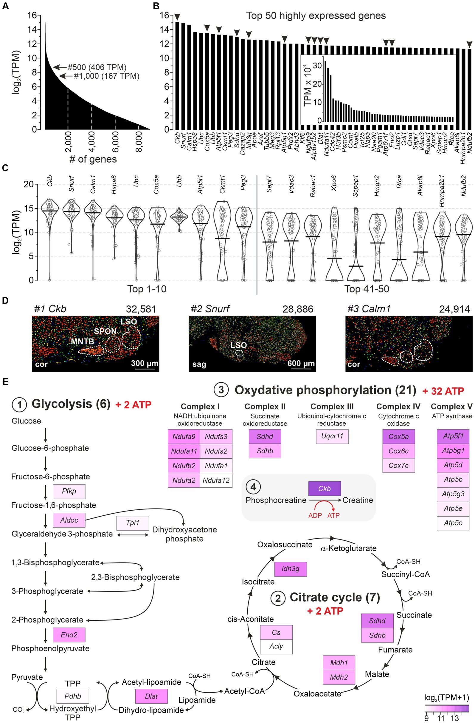
Highest gene expression levels imply high energy demands in LSO neurons

A major advantage of the single-cell patch-seq approach, which is absent from bulk analyses (Koehl et al., 2004; Nothwang et al., 2006; Ehmann et al., 2013; Xiao et al., 2013; Moritz et al., 2015; Kolson et al., 2016), is the ability to focus on neurons instead of globally addressing different cell types (including glia or blood endothelium). We took advantage of this and examined the most abundant transcripts in the 86 LSO neurons. Within the cohort of 9,082 genes with ≥1 TPM, 185 and 60 showed TPM values >1,024 and > 2,048, respectively (Figure 2A). The 50 most highly expressed genes are shown in Figure 2B (32,581–2,460 TPM, inset). For 20 of them, bee swarm and violin plots are depicted in Figure 2C. Three genes showed exceptionally high expression levels, namely Ckb, Snurf, and Calm1 (Figure 2B; mean TPM: 32,581, 28,886, 24,914). They encode brain-type creatine kinase B (CKB), SNRPN upstream open reading frame protein (SNURF; SNRPN = small nuclear ribonucleoprotein polypeptide N), and calmodulin 1 (CALM1 aka CaM), respectively. Our findings are corroborated by in situ hybridization results from the AMBA which show high signal intensities in the major nuclei of the superior olivary complex (SOC) (Figure 2D). Further information on Ckb, Snurf, and Calm1 is provided in the Discussion.

Figure 2. A majority of highly expressed genes reveal high energy demands for LSO neurons. (A) Expression levels of 9,082 genes with mean TPM ≥ 1 (log2). Arrows point to genes #500 and #1,000. (B) Top 50 highly expressed genes ranked by expression level. Arrowheads mark 13 genes involved in ATP synthesis (cf. E). (C) Violin plots for transcripts #1–10 and #41–50 from (B) (1 dot per neuron). Horizontal bars correspond to mean values. (D) In situ hybridization images of the SOC for the top three highly expressed genes (Ckb, Snurf, Calm1; modified images from AMBA; for URLs, see Supplementary Table S7). Expression mask image displays highlight cells that have the highest probability of gene expression (from low/blue to high/red). TPM values are also provided. (E) GSEA of the 500 most highly expressed genes (≥ 406 TPM). Three KEGG pathways: (1) Glycolysis (M00001, M00307), (2) Citrate cycle (M00009), (3) OxPhos (mmu00190). (4) ATP synthesis-related Ckb (#1). cor, coronal; sag, sagittal (see also Supplementary Table S2).

Glucose consumption is a signature of brain activity (Ashrafi and Ryan, 2017) and is particularly high in the CAS (Sokoloff, 1981). As 13 of the 50 most highly expressed genes in our sample encode enzymes involved in catabolism, we examined pathways of energy demand and ATP production in more detail. We analyzed gene enrichment in pathways that completely combust glucose to CO2 and H2O: (1) Glycolysis (including Pyruvate oxidation), (2) Citrate cycle, and (3) Oxidative phosphorylation (OxPhos; Supplementary Table S2). The analysis included 162 genes, including Ckb (4). Among the top 500 highly expressed genes, 7% (33) belonged into these pathways and were distributed across the four categories (Figure 2E). When normalized to the set of 162, the frequency was 20%. Taken together, these numbers emphasize and specify the genes involved in ATP generation and highlight the importance of energy metabolism in the LSO.

Gene enrichment analysis revealed seven genes among the top 500 that encode v-ATPase subunits (Atp6ap1, Atp6v1b2, Atp6v6v11, Atp6v0c, Atp6v0d1, Atpv1e1, Atp6v1d; 3,589–438 TPM; #24 to #460). Twenty-three v-ATPase genes have been described (Alexander et al., 2011). v-ATPases are associated with lysosomes and primary-active proton pumps which play an important role in driving transmitter loading into synaptic vesicles (Egashira et al., 2015). Our results indicate that LSO neurons were in a metabolically active state.

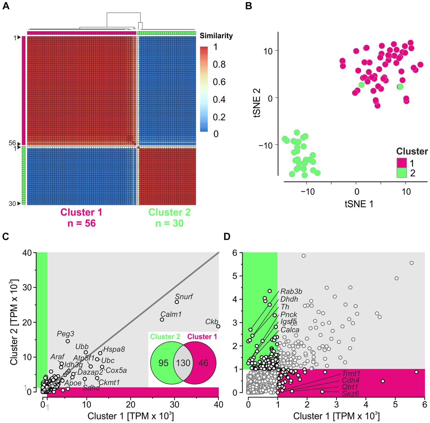
scRNA-seq reveals two clusters of LSO neurons

To identify neuron types in the LSO, we applied unsupervised clustering. We determined the consensus matrix for 2–10 clusters using SC3 and calculated the average silhouette width for each number of clusters (widths vary from 0 to 1; a width close to 1 represents the optimal number of clusters). We obtained the largest width (0.98) with two clusters (Supplementary Figures S3A,B). Fifty-six of the 86 neurons (~2/3) belonged to cluster 1, and 30 (~1/3) belonged to cluster 2 (Figure 3A). Similarity values were close to 1 for each neuron in its own cluster and close to 0 in the other cluster, except for neuron #1 in cluster 2. We checked for consistent results using the alternative tool Seurat, which assigned 59 neurons to cluster 1 and 27 neurons to cluster 2 (Supplementary Figure S3C). Fifty-six neurons in cluster 1 overlapped between SC3 and Seurat, while 27 neurons overlapped in cluster 2. The substantial overlap demonstrated consistency between the two tools. For three clusters, the results were less consistent and the overlap between SC3 and Seurat was small (Supplementary Figure S3D). Taken together, these results confirm the best results with two clusters.

Figure 3. Unsupervised clustering reveals two major clusters. (A) Consensus matrix obtained for two clusters. Matrix shows how often each pair of neurons (n = 86) is assigned to the same cluster (1 = 100%). (B) tSNE plot based on PCs 1–10. (C) Correlation analysis of global expression profiles for 11,659 genes. Magenta and green sections include non-intersecting genes with mean TPM ≥ 1,000 in cluster 1 and cluster 2, respectively. The top 15 highly expressed genes (cf. Figure 2B) are provided with names. Dots on the 45-degree line imply same gene expression levels in both clusters. Inset: Venn diagram showing the number of intersecting (Cluster 1 ∩ Cluster 2; n = 130) and non-intersecting genes (Cluster 1\Cluster 2) ∪ (Cluster 2\Cluster 1; n = 46 + 95 = 141). (D) Close-up of non-intersecting genes with ≥1,000 TPM (black dots). For genes with <100 TPM in the complementary cluster, names are provided (n = 4, 6) (see also Supplementary Figure S3).

To visualize the clustering results, we performed a PCA based on HVG (Methods and Supplementary Figure S3E). PC1 explained 11% of the variance and separated both clusters, except for two neurons belonging to cluster 2. Because PC1 plus PC2 together explained only 17% of the variance, we generated a tSNE plot using PC1–PC10. Again, the neurons were clearly separated into two clusters, except for two neurons (Figure 3B; see also Supplementary Figure S3E). Overall, these results demonstrate two major clusters for our sample, regardless of the clustering method used. Below, we explore the two clusters obtained by SC3.

After dividing the 86 patch-seq neurons into two clusters, we assessed the expression level of 11,659 genes (Figure 3C). Two hundred and seventy-one genes exceeded TPM ≥ 1,000 in at least one cluster. Approximately 50% of the genes overlapped (130/271; inset), indicating considerable similarity between the two clusters. Each of the 13 genes involved in ATP synthesis shown in Figure 2B ended up in the intersection, suggesting high metabolic demands in both clusters. Among the 141 non-intersecting genes with ≥1,000 TPM (46 in cluster 1; 95 in cluster 2), only four and six, respectively, showed <100 TPM in the complementary cluster (Figure 3D). This again indicates homogeneity between the two clusters for many transcripts.

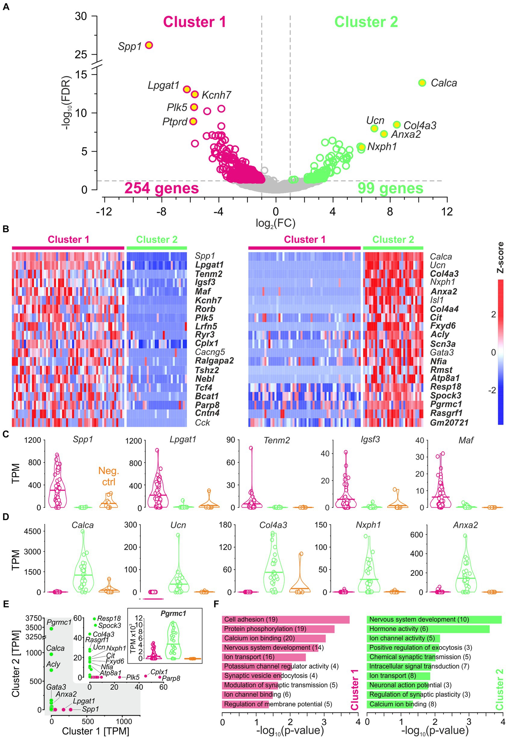
Search for molecular signatures in each cluster

The above comparisons revealed considerable similarities between the clusters. To identify differences, we focused on DEGs (see Methods for definition). As documented in a volcano plot, 353 DEGs were identified, of which 254 were upregulated in cluster 1 and 99 in cluster 2 (Figure 4A; Supplementary Table S3). To identify the top DEGs, the DEGs were ranked by the AUROC value. In Figure 4B, the expression of the top 40 DEGs, 20 in each cluster, is visualized in heatmaps (56 neurons in cluster 1, 30 in cluster 2). Below and in Supplementary results, we provide some background information for each of these top 40 DEGs.

Figure 4. DEGs affiliate cluster 1 with pLSOs and cluster 2 with LOCs. (A) Volcano plot depicting DEGs for each cluster. DEGs#1–5, as ranked by FC values, are provided with names (yellow dots). Dashed gray lines depict cut-off levels (FC = 2; FDR = 0.05). (B) Heat maps of z-scores for the top 20 DEGs in each cluster. Thirty-two newly detected genes are marked in bold. (C) Violin plots for DEGs#1–5 in cluster 1 (magenta). Horizontal bars depict mean values. Values from cluster 2 (green) and negative controls (orange) are shown for comparison. (D) As (C), but for cluster 2. (E) Scatter plot comparing the median expression levels of DEGs#1–20 from cluster 1 and 2. Inset is a close-up for ≤60 TPM. Genes with >10 TPM are provided with names (5 in cluster 1, 15 in cluster 2). Violin plot for Pgrmc1, DEG#18 in cluster 2. (F), Selected enriched GO terms for DEGs in cluster 1 (magenta) and in cluster 2 (green). Number of genes in brackets (see also Supplementary Tables S3, S4).

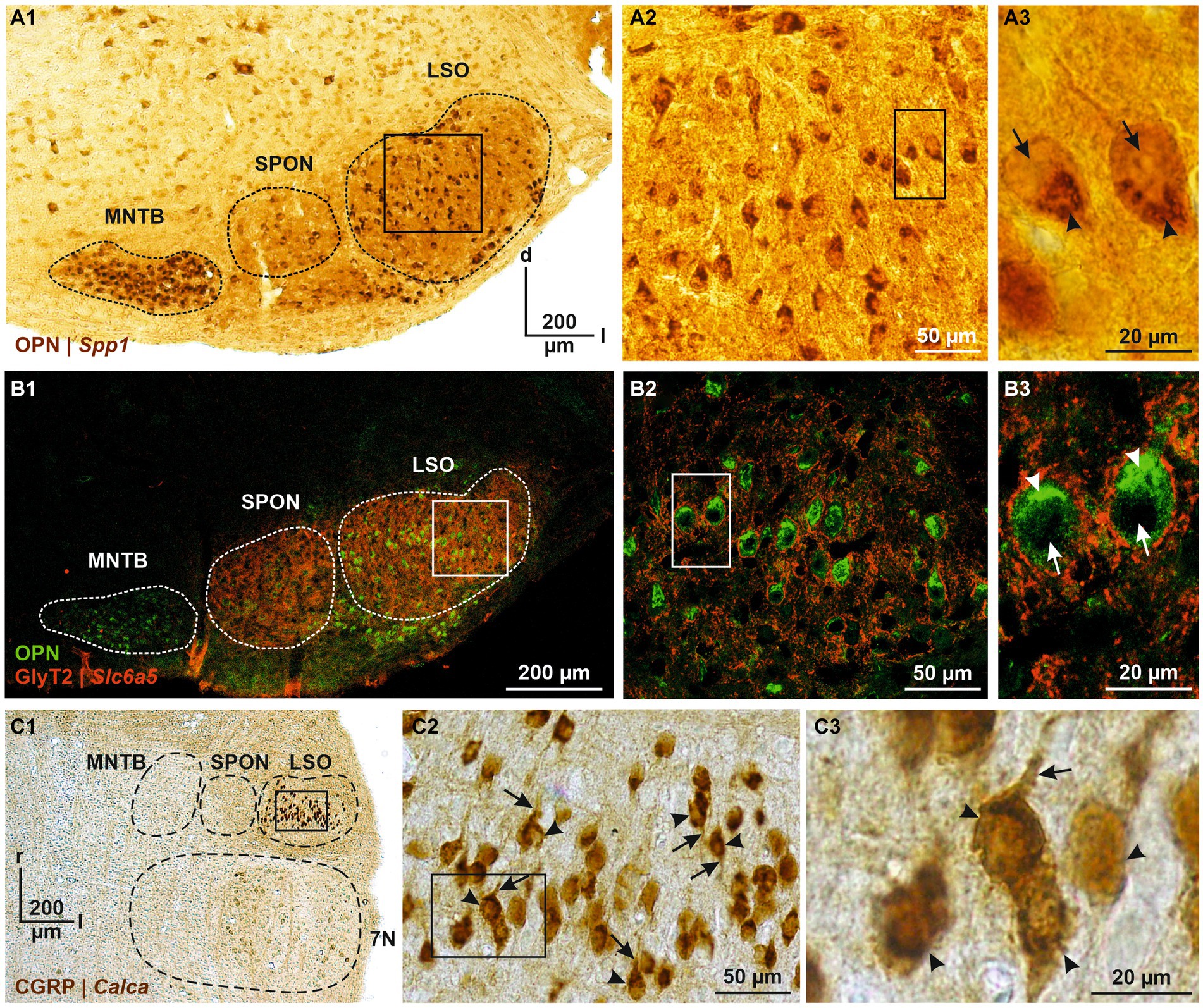
Cluster 1, DEGs#1–6 #1—Spp1: osteopontin

DEG#1 in cluster 1 was Spp1 (Figures 4B,C,E). Spp1 codes for the secreted phosphoprotein 1 = osteopontin (OPN), a cell adhesion molecule with multiple functions (Denhardt and Guo, 1993). Its expression is reported to be high in >20 brainstem regions, and OPN mRNA has been described in some LSO neurons of P14 rats (see Figure 3C in Lee et al., 2001). Our results from P11 mice are consistent with this pattern (see Figures 5A,B). In the rat cochlear nuclear complex, Spp1 expression resulted in 5-14-fold higher mRNA levels in the two ventral nuclei than in the dorsal nucleus (see Figure 5 in Friedland et al., 2006). Spp1 contributes to neuronal development (Jiang et al., 2019), including axon myelination (Selvaraju et al., 2004; Nam et al., 2019; Cappellano et al., 2021) and axon regeneration after injury (Duan et al., 2015). It has been suggested that OPN is involved in the formation and/or maintenance of axons with high conduction velocity (Higo et al., 2010). Notably, pLSO and MNTB neurons are myelinated (as are neurons in the ventral cochlear nuclei and motoneurons), whereas LOCs are not. The AMBA shows high to intermediate expression levels for Spp1 in the LSO at P14 and at P56 (Supplementary Figure S4). Corresponding immunohistochemical views of the OPN protein pattern are shown in Figures 5A,B. For Spp1 and subsequent genes, the expression level and numerical details are provided in Supplementary Table S3. In summary, our Spp1|OPN results support the idea that pLSOs belong to cluster 1, whereas LOCs do not.

Figure 5. Immunohistochemical analysis of OPN and CGRP, encoded by DEG#1 in cluster 1 and cluster 2 (Spp1 and Calca, respectively). (A1) OPN immunoreactivity in the SOC (A1, coronal brainstem section) and LSO (A2). DAB-stained coronal brainstem slice at P12. Close-up of two representative neurons in (A3). (B) As (A), but double labeling for OPN (green) and GlyT2 (red). In (A3,B3), cytoplasmic immunosignals are marked by arrowheads and nuclei by arrows. (C) CGRP immunoreactivity in the SOC (C1, horizontal brainstem section) and LSO (C2). DAB-stained horizontal brainstem slice at P12. Close-ups of four representative neurons in (C3). In (C2,C3), somatic and dendritic immunosignals are marked by arrowheads and arrows, respectively. Borders of MNTB, SPON, 7 N, and LSO are indicated by dashed black or white lines. d, dorsal; l, lateral; r, rostral; 7 N, facial nucleus.

#2—Lpgat1: lysosphatidylglyceral acyltransferase 1

DEG#2 in cluster 1 was Lpgat1 (Figures 4B,C,E). This gene codes for lysophosphatidylglycerol acyltransferase 1 (LPGAT1), an enzyme associated with the endoplasmic reticulum and involved in lipid metabolism (Yang et al., 2004). LPGAT1 regulates triacylglycerol synthesis which is critical to maintain the integrity of mitochondrial membranes (Wei et al., 2020). In the vestibular organ of chickens, the protein has been exclusively identified in hair cells (Herget et al., 2013). The AMBA shows high Lpgat1 expression in the LSO at P56 (Supplementary Figure S4, no AMBA data available for P14).

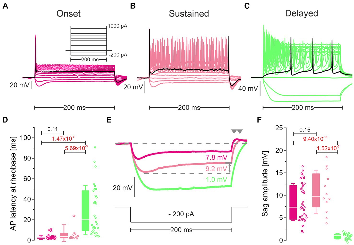
Figure 6. Cluster 1 neurons and cluster 2 neurons differ in their firing pattern and their response to hyperpolarization. (A–C) Representative voltage traces in response to rectangular current pulses (inset in A; −200 to +1,000 pA, 100 pA increments, 200 ms duration) of an onset firing cluster 1 neuron (pLSO—Onset; (A), a sustained firing cluster 1 neuron (pLSO—Sustained; (B), and a delayed firing cluster 2 neuron (LOC—Delayed; (C). Black traces depict responses at rheobase. Notice different voltage scaling. (D) Statistics for the peak latency of the first AP at rheobase. Open dots depict single neurons. Numbers above bars represent p-values (in red if significant). (E) Voltage traces in response to a − 200-pA|200-ms current pulse highlighting sag behavior. Same color code as in (A–C). Sag amplitudes were quantified as indicated by the gray double arrow. Rebound behavior after the hyperpolarizing current pulse is marked by gray arrowheads. (F) As (D), but for sag amplitude (see also Supplementary Table S5).

#3—Tenm2: teneurin transmembrane protein 2

DEG#3 in cluster 1 was Tenm2 (Figures 4B,C). Tenm2 belongs to the teneurin family that comprises four members (Tenm1-4). It codes for teneurin transmembrane protein 2 (TEN2, aka TENM2), an axon guidance and adhesion molecule that interacts across the synaptic cleft with presynaptic latrophilin1, thus mediating Ca2+ signaling and synapse formation (Vysokov et al., 2016). Teneurin proteins are abundant throughout the central nervous system and play a role in regulating synaptic partner matching (Hong et al., 2012; Leamey and Sawatari, 2014). A distinct role of Tenm2 in the generation of binocular projections has been demonstrated in the mouse visual system, and Tenm2 knockout resulted in specific wiring deficits in the retinogeniculate pathway (Young et al., 2013). In the auditory system, high Tenm2 expression is present in spiral ganglion neurons of the Ib subtype, whereas type II neurons highly express Tenm3 (Petitpré et al., 2018). As to date, information about Tenm2 in the CAS is missing. The AMBA shows a few cells with low Tenm2 expression in the LSO at P56 (Supplementary Figure S4, no AMBA data available for P14).

#4—Igsf3: immunoglobulin superfamily member 3

DEG#4 in cluster 1 was Igsf3 (Figures 4B,C). It belongs to the Ig superfamily whose members are major regulators of many developmental processes, such as differentiation, axogenesis, dendritogenesis, and synaptogenesis. Like the other three members of the little studied EWI Ig subfamily, IGSF3 (aka EWI-3) contains a Glu-Trp-Ile (EWI) motif. IGSF3 is a neuron-specific membrane protein that is produced in various neuronal populations when neural circuits are formed (Usardi et al., 2017). It is transiently found in cerebellar granule cells before their final maturation and highly concentrated in axon terminals. The AMBA shows only two cells expressing Igsf3 in the LSO at P56 (Supplementary Figure S4, no AMBA data available for P14).

#5—MAF: MAF bZIP transcription factor

DEG#5 in cluster 1 was Maf (Figures 4B,C). The Maf family encodes b leucine zipper (bZIP)-containing transcription factors which act as homo-or hetero-dimers. Depending on the binding site and binding partner, the encoded proteins are transcriptional activators or repressors. cMAF controls eye and lens development (Ring et al., 2000) and directs the development of low-threshold touch receptors (Wende et al., 2012). Pacinian corpuscles, which are essential to detect small-amplitude high-frequency vibrations, become severely atrophied in c-Maf mutants. Several genes encoding K+ channels are downregulated in such mutants (Kcna1, Kcng4, Kcnh5, Kcnq4). In the cerebral cortex, c-MAF regulates the potential of GABAergic interneurons to acquire a somatostatin-positive identity, shortly after these neurons become postmitotic (Mi et al., 2018). The AMBA shows high expression levels for Maf in the LSO at P14 and at P28 (Supplementary Figure S4).

#6—Kcnh7: potassium voltage-gated channel subfamily H member 7

DEG#6 in cluster 1 was Kcnh7 (Figure 4B). Kv11.3, the encoded protein, is the third member in the family of ERG channels (ether-a-go-go-related). Our study demonstrates no gene expression for Kv11.2 and only low expression for Kv11.1 (cf. chapter “Potassium channels”). Consistent with our results, the AMBA shows low to intermediate Kcnh7 expression in the LSO at P14 and P56 and few cells with high signal intensity at P56 (Supplementary Figure S4). Below, we further analyze Kcnh7|Kv11.3 on the protein level (cf. chapter “Immunohistochemical analysis of Kv11.3 and Kvβ3”), and we refer to the Discussion for an elaborate treatise.

#7–20

Information on DEGs#7–20 is provided in Supplementary results.

Cluster 2, DEGs#1–6 #1—Calca: calcitonin gene-related peptide

DEG#1 in cluster 2 was Calca (Figures 4B,D,E). Calca codes for CGRP, the calcitonin gene-related peptide. As elaborated in the Introduction, CGRP is present in LOCs but absent from pLSOs. Therefore, our DEG results provide initial hints that cluster 2 may comprise LOCs. To assess whether the protein follows mRNA, we performed immunohistochemical analysis of CGRP and demonstrated intense labeling in the LSO (Figure 5C), therewith confirming previous results (Safieddine and Eybalin, 1992; Robertson and Mulders, 2000). AMBA shows LSO cells with high gene expression at P14 and intermediate to high expression at P56 (Supplementary Figure S5).

#2—Ucn: urocortin

The tentative conclusion that cluster 2 comprises LOCs was reinforced by our findings on DEG#2, which was Ucn (Figures 4B,D,E). Ucn codes for urocortin, one of three members in the urocortin family composed of stress-related corticotropin-releasing hormone neuropeptides. In rats, urocortin was demonstrated in a small subset of LSO neurons (Vaughan et al., 1995; Kaiser et al., 2011). It is reportedly absent from other auditory nuclei (Bittencourt et al., 1999). Ucn expression appears to be specific for LOCs, and urocortin is abundant in their axon terminals in the cochlea (Vetter et al., 2002; Kaiser et al., 2011). Consistent with our results, AMBA shows LSO cells with high gene expression levels at P14. Interestingly, Ucn expression P56 is almost absent (Supplementary Figure S5). As LOCs modulate the excitability of auditory nerve fibers, urocortin may balance physiological reactions to acoustic stress via high affinity binding to corticotropin-releasing factor receptor CRFR1 during development (Graham and Vetter, 2011).

#3—Col4a3: collagen type IV alpha 3 chain

DEG#3 in cluster 2 was Col4a3 (Figures 4B,D,E). Col4a3 codes for the α3 domain of type IV collagen. Type IV collagens are the major structural component of basement membranes, including the strial capillary basement membranes in the inner ear. Col4a3 mutations affect the structure and function of the cochlea and result in syndromic deafness (Mochizuki et al., 1994; Angeli et al., 2012; Kolla et al., 2020). Thus, Col4a3 is considered a deafness gene (Müller and Barr-Gillespie, 2015). As to date, the literature is virtually devoid of reports on Col4a3 in combination with neurons. Type IV collagens inhibit cell proliferation and astroglial differentiation while promoting neuronal differentiation (Ali et al., 1998). In this context, it is of some interest that DEG#7 in cluster 2 was Col4a4, which encodes the α4 domain of type IV collagen (Figure 4B). AMBA shows low Col4a3 expression in a few cells in the LSO at P56 (Supplementary Figure S5, no AMBA data available for P14). However, Col4a3 was identified very recently as a marker for LOCs in a study that employed single-nucleus sequencing in mice (Frank et al., 2023). Our results confirm these findings.

#4—Nxph1: neurexophilin 1

DEG#4 in cluster 2 was Nxph1 (Figures 4B,D,E). Nxph1 codes for the neuronal glycoprotein neurexophilin1. Four isoforms of neurexophilin (Nxph1-Nnxph4) form a conserved family of neuropeptide-like molecules that interact with neurexins, crucial presynaptic cell-adhesion molecules (Missler and Südhof, 1998; Ding et al., 2020). Nxph1 is a specific ligand for α-neurexin 1 (aka NRXN1α) and essential for transsynaptic activation. Neurexins (NRXN1-3) consist of an α-and a β-protein and play important roles in synaptic plasticity and synapse maturation. By binding to the postsynaptic ligand, they can directly influence ligand-binding receptors, thereby altering a neuron’s excitatory or inhibitory ability. A restricted Nxph1 expression was described in subpopulations of inhibitory neurons (Petrenko et al., 1996; summary: Born et al., 2014). Conjunctively, these transsynaptic cell adhesion molecules coordinate synapse formation, restructuring, and elimination in both directions. From in the Petrenko paper, one can deduce that LSO neurons express neurexophilin. AMBA shows a low to intermediate expression level in the LSO at P56 (Supplementary Figure S5, no AMBA data available for P14).

#5—Anxa2: annexin A2

Anxa2, DEG#5 in cluster 2 (Figures 4B,D,E), is one of 13 annexin A genes expressed in vertebrates. Members of this subfamily are soluble proteins that are recruited to membranes in the presence of elevated Ca2+ where they bind phospholipids. Among the multiple roles of annexins are membrane aggregation, exocytosis, and endocytosis regulation. Anxa2 is highly expressed in nociceptors where AnxA2 regulates TRPA1-dependent acute and inflammatory pain (Avenali et al., 2014). Gene expression was also demonstrated in surrounding cells in the developing mouse cochlea (Scheffer et al., 2015). To our knowledge, relevant papers on auditory neurons do not exist (Pubmed search: “Anxa2 auditory” or “Annexin A2 auditory”; 2023–10-22). AMBA shows only a few LSO cells with low Anxa2 expression at P14 and P56 (Supplementary Figure S5).

#6—Isl1: insulin gene enhancer protein ISL1

Isl1 (aka Islet-1), DEG#6 of cluster 2 (Figure 4B), is a homeobox gene encoding the insulin gene enhancer protein ISL1. The gene product, a transcription factor, promotes motoneuron development (Ericson et al., 1992) and affects efferents to the inner ear. Isl1 expression has been reported in olivocochlear efferents (Frank and Goodrich, 2018). Our patch-seq results are consistent with these reports. As the inner ear efferents originate in a progenitor zone for motoneurons, it is not surprising that factors assigning a motoneuron identity (e.g., ISL1 and ChAT) overlap considerably between such efferents and facial motoneurons. In fact, inner ear efferents represent a subset of motoneurons, although they form no synapses with muscle fibers (Frank and Goodrich, 2018). AMBA shows few LSO cells with intermediate to high Isl1 expression at P56 (Supplementary Figure S5, no AMBA data available for P14).

#7–20

Information on DEGs#7–20 is provided in Supplementary results.

Summary for DEGs#1–20 of each cluster

Taken together, DEGs#1–20 in cluster 1 plus cluster2 contain eight genes (20%) whose expression was previously described in the LSO (cluster 1: Spp1, Cacng5, Cck; cluster 2: Calca, Ucn, Nxph1, Isl1, Gata3). We now attribute their expression to neurons. The results for the remaining 80% of the genes are new. Each of the three known DEGs in cluster 1 can be associated with pLSOs. Similarly, four genes from cluster 2 can be associated with LOCs (Calca, Ucn, Isl1, Gata3). Thus, the transcriptomic results provide substantial and consistent evidence to conclude that cluster 1 and cluster 2 contain pLSOs and LOCs, respectively. If our conclusion is correct (see below), we identified 17 novel marker genes for pLSOs and 15 for LOCs (highlighted in bold in Figure 4B).

Figure 4B shows 40 DEGs ranked by the z-score. Corresponding expression levels are detailed in violin plots (Figures 4C,D), highlighting significant expression differences. We also plotted the corresponding TPM values for both clusters (Figure 4E and inset