The proper orientation of cells with regard to anatomical axes, neighboring cell orientation, and overall system organization is of critical importance for proper development and function in nearly all multicellular organisms. During metazoan development, immature sheets of cells respond to polarization cues that provide the organizational direction necessary for the formation of complex tissues, organs, and systems. The study of coordinated cell polarization in these two dimensional sheets—known as planar cell polarity (PCP)—has greatly benefitted from the improvement of molecular and gene targeting methodology developed over the past few decades, and there has been considerable scientific interest in studying PCP pathways in a variety of developing tissues and model organisms (López-Schier et al., 2004; Classen et al., 2005; Djiane et al., 2005; Dohn et al., 2013; Wang et al., 2016; Yang et al., 2017). Indeed, several factors that regulate PCP have been identified, including several “core” PCP proteins that appear to be largely conserved (Seifert and Mlodzik, 2007; Dreyer et al., 2022). In addition, several recent publications show that there are novel PCP factors to be discovered (Bonello and Peifer, 2019; Landin Malt et al., 2019), some that may be specific to certain tissue types or species (Hale and Strutt, 2015; Pitsidianaki et al., 2021). There is also a growing list of functions for many PCP proteins beyond mere polarization (Cheong et al., 2020; Humphries et al., 2020). As this area of study continues to grow, new tool development and adoption of streamlined methodologies will be highly beneficial.

A major technical limitation in the study of PCP is that the manual characterization and collection of cellular polarity data is incredibly labor intensive. Most types of tissue contain thousands-to-millions of cells, making it nearly impossible to conduct analyses on the entire cell population within an organ. Many investigators elect to quantify cell orientations from a limited number of sampling areas or cells and then extrapolate broader regional conclusions based on this data. Even with such random and limited sampling, statistical power and experimental rigor often require the measurement of hundreds of cells, which is still intensive and vastly time consuming for investigators taking manual measurements. Furthermore, limited sampling techniques may lead investigators to draw incorrect regional assumptions, particularly in cases where cell type ratios or cell density varies based on anatomical location (Desai et al., 2005) or developmental age (Burns et al., 2012). Beyond the extensive time commitment necessary to collect PCP data, manual quantification of planar cell polarity—even by blinded investigators—is subject to human error and potential bias. Due to the limitations inherent in manual cell quantification, there has been a growing interest in the development of automated or semi-automated processes that would allow researchers to collect PCP data quickly and accurately. Automation of PCP data collection should provide tremendous savings in terms of time and human resources, with the added benefit of minimizing variability and bias.

To address the need for a reliable and user-friendly approach to automating PCP data collection, we have developed a user-friendly plug-in tool suite called PCP Auto Count (PCPA). PCPA automates cell quantification and collects PCP data in the form of angle measurements from two-dimensional micrographs. PCPA is integrated with the widely used open-source software Fiji (Fiji Is Just ImageJ) (Schindelin et al., 2012) and allows researchers to customize data collection parameters through a simple graphical user interface. To test the efficacy of PCPA we utilized a number of confocal fluorescent micrographs taken from murine inner ear sensory epithelia and compared data collected with PCPA against data collected through traditional manual quantification methods.

Inner ear auditory and vestibular sensory epithelia have become prominent models for the investigation of how disruption to developmental factors can affect PCP (Landin Malt et al., 2019; Kozak et al., 2020; Ohta et al., 2020). The main sensory cell type of the inner ear—known as hair cells—are characterized by stereocilia protruding from the apical surface of the cell which are pushed by mechanical forces in the direction of the cell’s primary cilium or kinocilium. When this deflection is properly aligned mechano-electric transduction channels are opened, depolarizing the cell and triggering neurotransmitter release onto the vestibulocochlear nerve. In order to be maximally sensitive to deflecting forces, sensory hair cells develop specific spatial orientations during late embryonic and early postnatal ages. Disruption to developmental factors influencing PCP have been shown to lead to deficits in hearing and balance (Duncan et al., 2017; Tarchini, 2021; Ji et al., 2022). Thus, we have developed the PCPA plug-in suite to automate the collection of cell polarity measurements and validated its utility extensively in cochlear and vestibular sensory epithelia. In addition, we demonstrate the ability of PCPA to obtain orientation measurements from published images of Drosophila ommatidia, murine ependymal cells, and murine radial glia. Together, the data suggest that PCPA is a reliable and accurate plug-in suite that performs at least as well as manual quantification, and has significant potential to streamline and expand planar cell polarity analyses in multiple cell types and tissue models.

Finally, though the PCPA plug-in was primarily developed to calculate cell polarity measurements, it also provides broader experimental applicability through its ability to quantify cell numbers. Across many areas of study in the biological sciences, the counting of cells is necessary to understand the effects of experimental manipulations. Investigators often wish to quantify changes in RNA or protein expression in situ, or on the processes of cell survival, proliferation, and differentiation by counting cells expressing certain markers. In the inner ear, sensory cells can be damaged or lost due to environmental factors, genetic predisposition, and the normal aging process. Many research questions related to sensory cell protection or regenerative strategies use cell population counts as an important outcome metric, and this approach (Kaltenbach et al., 2002; O’Sullivan et al., 2020; Ciani Berlingeri et al., 2022) is subject to the same limiting factors described above (time investment and potential bias). Though not heavily emphasized here, our results demonstrate that PCPA can be used to quantify cell numbers in addition to angles of orientation, or independently for samples where cell polarity information is not needed.

The PCPA plug-in requires no special licensing or permission to use, and runs on any operating platform supported by Fiji (i.e., Linux, Windows, MacOS). The PCPA plugin can be found at https://sites.imagej.net/PCP-Auto-Count/. Detailed instructions for installing Fiji plug-ins can be found in the PCPA user manual or through Fiji’s wiki at https://imagej.net/plug-ins/updater or https://imagej.net/plug-ins/. A user manual with detailed explanations of the PCPA algorithm and function, along with PCPA’s open source code, can be found at https://github.com/WaltersLabUMC/PCP-Auto-Count.git.

For P4 cochlear images obtained using optimal microscopy parameters described above, we found that further pre-processing was often not necessary and we could move straight to creating binary images from these micrographs. For any images that did not meet the criteria defined above (high SNR and flat 2D image), we found that pre-processing steps completed using existing features in Fiji enhanced the quality of subsequently created binary images, and ultimately resulted in nearly all positively labeled cells from the micrographs to be processed successfully by PCPA. We briefly describe the preprocessing steps used below, and a detailed explanation of pre-processing settings can be found in the PCPA user manual which can be obtained within the PCPA plug-in (or at https://github.com/WaltersLabUMC/PCP-Auto-Count.git).

First, to create 2D images from 3D (z-stack) micrographs, the Fiji function “Image > Stacks > Z project … ” allowed for projection using a variety of methods. Of these, the maximum intensity projection worked best for most images, though the median intensity function sometimes yielded better results. In cases where SNR was low, PCPA performance was improved by selecting “Process > Subtract background … ”. Standard Fiji functions were not always sufficient to correct high heterogeneity of signal within particularly poor images. In these cases, we corrected image intensity using the BioVoxxel plug-in tool suite (www.biovoxxel.de). Specifically, the “pseudo flat-field correction” option and/or “convoluted background subtraction” option improved homogeneity of signal intensities and allowed further background subtraction if needed after flat-field correction. After background subtraction (if applicable), images were converted to binary, most commonly by using the Fiji function “Image > Adjust > Threshold … ,” where users manually set the threshold point. Alternatively, for images that were of sufficient quality and homogeneity, Fiji’s automated threshold options could be used (e.g., “Process > Binary > Make Binary”).

When making an image binary, nonspecific staining could be intense enough to be included as white pixels. While distinct non-specific white pixels can be size excluded (via PCPA’s size exclusion settings, described below), white pixels that arise in direct contact with cells of interest could lead to erroneous calculations of the centers of the cells during PCPA analysis. Furthermore, it is generally beneficial to PCPA processing to eliminate spurious concavities from cells, i.e., any indentations or holes that are not the feature to be measured for directionality. While allowing such features to remain would likely only slow PCPA analysis by a few seconds, it could lead to occasionally erroneous angle measurements. Thus, it is highly recommended to use the Fiji option “Process > Noise > Remove outliers … ” to remove these non-specific features. For the images used in this report, noise removal between 6–12 pixels was generally sufficient.

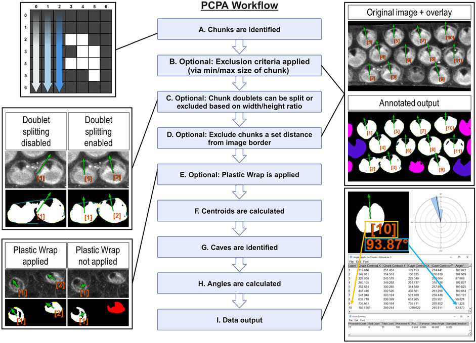
Here, we provide a brief description of PCPA’s workflow and algorithmic processes, presented in operational order (Figure 1) PCPA will first identify all potential chunks in a binary image. To do so, the Cartesian (x, y) coordinates of all white pixels in the image are recorded. PCPA then systematically evaluates every white pixel to determine if it abuts any other white pixels. All abutting pixels are assigned as an aggregate representing an individual chunk (Figure 1A). The coordinates of all chunk pixels are then stored for later use in calculating the center of mass of each chunk. PCPA then discards any chunks violating optional size exclusions from further analysis. The user-defined upper and/or lower size limits (Supplementary Figure S1A) allows users to filter out spurious signal and to select for cells in a size range, which can be particularly useful for filtering out immature cells which may not have yet developed sufficient PCP characteristics for proper analysis (Figure 1B).

Figure 1. Overview of PCPA’s algorithmic flow (Created with BioRender.com) (A) PCPA identifies aggregates of white pixels in a binary image, termed chunks. (B) Chunks can be discarded from subsequent operations via an optional pixel size minimum and/or maximum (cells pseudo-colored pink). (C) PCPA has a limited capacity (maximum of two conjoined cells) to separate chunks that abut one another or overlap. Larger aggregates of chunks can be excluded by overall size or dimensions. (D) Cells that fall partially outside of the imaging frame can be discarded by setting an exclusion zone of a set number of pixels away from the edge of the image frame (cells pseudo-colored blue). (E) In the absence of Plastic Wrap, indentations in the chunk that are not completely enclosed by white pixels cannot be recognized by PCPA. Applying the “Plastic Wrap” option will add pixels to bridge the gap in the cell’s perimeter thus enclosing the indented area. (F) Each chunk’s center of mass is calculated and stored as (x, y) coordinates. (G) Inclusions of black pixels within chunks, or created by plastic wrap, termed caves, are identified and the cave best meeting selection criteria is identified as the directional cave of interest and the center of mass of the enclosed black pixels is calculated as (x, y) coordinates. (H) The angle of orientation for each chunk and its cave is calculated as the inverse tangent of the difference in (y) over the difference in (x). (I) PCPA outputs include annotated images specifying chunks excluded due to violating chunk size limits (cells pseudo-colored pink) or touching the border of the image (cells pseudo-colored blue). Cells are labeled in the annotated output and correspond with the angle results table, which provides a detailed output of (x, y) coordinates and angles for each chunk-cave pair that was quantified. Rose diagrams and summary statistics tables are also produced.

As the fusion of neighboring cells in micrographs is a common problem in automated image analysis (Courtney et al., 2021; Salazar et al., 2022; Sung et al., 2022), we developed an optional Doublet Splitting mode, where PCPA will separate two cells that touch or overlap by splitting the doublet mass in half, then treating each half as a discreet cell during subsequent steps (Supplementary Figure S1B). This optional function cannot recurse beyond separating two conjoined cells. and works most effectively when fused cells are somewhat reasonably aligned with the x or y-axis of an image. In this way, users can avoid having to manually separate all conjoined cells in an image. Alternately, users can choose to discard all doublets (triplets, or larger aggregates) from further analyses via size exclusion if preferred (Figure 1C). After PCPA has applied any optional doublet splitting or excluded aggregate cells, PCPA will then optionally exclude cells a set distance from the image border (Supplementary Figure S1A). Setting a border exclusion zone is recommended as this allows users to filter out cells that did not completely enter the imaging frame. PCPA then calculates a center of mass for all logged chunks by calculating the average x and y values for all of the pixels within a chunk and stores this information for later PCP angle measurement calculations (Figure 1F).

A cave is defined as any black pixel, or aggregate of black pixels, fully contained within the body of a chunk (i.e., completely surrounded by white pixels constituting the chunk). If the primary PCP-indicating features present as unenclosed indentations (e.g., the u-shaped configuration of rhabdomeres in Drosophila ommatidia), we developed an optional feature called Plastic Wrap to enclose such concavities (Supplementary Figures S2A-S2A’). Plastic wrap identifies any breaks in the arc of a chunk’s perimeter due to indentations in the chunk, then subsequently adds a one-pixel thick bridging line across these areas (Figure 1E). Algorithmically, Plastic Wrap runs immediately prior to chunk centroid calculations because the bridging pixels added by Plastic Wrap are considered part of the cell mass for subsequent chunk centroid calculations. For a more in-depth explanation of Plastic Wrap, see the PCPA user manual or source code.

Because natural cell variation, or due to loss of detail during the process of making binary images, or due to the application of Plastic Wrap, a chunk may contain more than one cave. PCPA must identify one cave to serve as the directional marker of interest for angle calculations. PCPA will first compile the coordinates of all caves (including any caves created by Plastic Wrap) in each chunk. PCPA will then select the cave that best meets user-defined criteria to be designated as the directional point of interest. Users may set the largest cave in the chunk or the cave best meeting a directional criterion (i.e., northmost, etc.; Supplementary Figures S2C-S2C’) as the selection criteria for the directional marker of interest. This selection criteria can be combined with optional cave minimum and/or maximum size requirements, which will exclude any caves violating size requirements prior to cave of interest selection (Supplementary Figure S2B). PCPA will then calculate the center of mass for the cave of interest to use for subsequent PCP angle calculations (Figure 1G).

PCPA will calculate the inverse tangent of the chunk and cave centers of mass for each chunk/cave pair in the image (Figure 1H). Angle measurements can be calculated on a −180°/180° or 0°/360° axis where angles increase incrementally clockwise or counter-clockwise. Users are able to customize their axis settings in the PCPA options dialogue (Supplementary Figure S3A).Once angle measurements have been calculated, PCPA will output data tables and annotated images, explained as follows (Figure 1I). The Results Table consists of a data row for each chunk analyzed and contains: an identification number assigned to each chunk, the (x, y) coordinates of the chunk, and the angle measurement of the chunk-to-cave vector. The Chunk Summary table contains summary statistics for the data set, including: Processed Count (the number of cells where an angle was measured), Bad Count (the number of cells for which no angle was measured), Total Count (sum of Processed Count and Bad Count), Processed %, mean angle, resultant mean length (RML), circular variance, and circular standard deviation. The output also includes a circular data histogram known as a rose or windmill diagram. The Successfully Processed Chunks output image features annotations superimposed onto the binary image used for analysis, and includes each cell’s identification number, angle measurement, and a directional arrow derived from the angle measurement. This output also features pseudo-coloring to indicate if any chunks were excluded from analysis and why. Pseudocolor designations can be customized by the user so that each exclusion category is color specific (Supplementary Figure S4E). Lastly, an overlay image containing only the identification number, angle measurement, and directional arrow for all analyzed cells in the image is produced. This overlay image can be superimposed over top the original grayscale or color micrograph using inbuilt Fiji functionality (“Image > Overlay > Add image … Zero transparent”). Each of these outputs can be selected or deselected by users in the PCPA options dialog (Supplementary Figure S4A).

While the aforementioned functionality described above constitutes the main intended use of PCPA analysis using a single binary image, PCPA has two further functionalities of note. Firstly, PCPA can batch process multiple binary images, aggregate each image’s cell measurements into one data set, then produce a Results Table, Chunk Summary Table, and rose diagram for this data set. This functionality allows users to quickly and easily calculate a comprehensive PCP data set for all sample micrographs of an experimental group taken from the same region. Second, the PCPA plug-in suite also contains a stand-alone rose diagram feature which allows users to input any numerical angle measurement dataset to obtain descriptive circular statistics and a rose diagram, regardless of whether or not the data set was collected via PCPA. Step-by-step instructions for using batch processing and the standalone rose diagram function can be found in the PCPA user manual.

To obtain utricles from embryonic day (E) 17.5 mice, a timed mating strategy was employed to cross Six2(+/−) female mice with Six2(+/−) males. The Six2(+/−) mice were created and maintained as a mixed background of C57Bl/6J and 129/Sv (Self et al., 2006). The male and female mice were paired in the evening, and on the following morning the male was removed and female mice were assumed pregnant with embryos at stage E0.5. On day E17.5, dams were euthanized and embryos were collected. The heads of the embryos were removed, rapidly hemi-sectioned, then placed into 4% paraformaldehyde for 4 h at room temperature (RT) then stored in PBS at 4°C until use. Tail biopsies were collected into sterile microcentrifuge tubes for genotyping. Only wild type embryos were utilized for PCPA data collection. For postnatal cochlea experiments, CD1 mice were euthanized at postnatal day (P) four and temporal bones were collected into 4% paraformaldehyde for 4 h at RT then stored in PBS at 4°C until use.

P4 cochlear whole mounts were washed in PBS then incubated in Image-iT™ FX signal enhancer for 30 min at RT. Following PBS washes, samples were immersed in blocking buffer (0.2% Triton-X and 4% donkey serum) for 60 min at RT. The Mouse on Mouse (M.O.M.) IgG Blocking Reagent kit was used per manufacturer’s instructions and the following primary and secondary antibodies were used: anti-Pou4f3 (1:200), anti-βII-spectrin (1:200), Alexa Fluor 647 goat anti-mouse IgG1 (1:1,000), Alexa Fluor 568 goat anti-mouse IgG1 (1:1,000), Alexa Fluor™ 488 Phalloidin (1:800), and Hoechst 33,342 (1:1,500). Following a final PBS wash, samples were mounted with Fluoro Gel with DABCO. A detailed list of all antibodies and reagents used, including catalog and RRID numbers is presented in Supplementary Table S1. Z-stack images of cochlear hair cells were taken from randomly selected areas from the apex, middle, and base of P4 cochleae using a Zeiss LSM 880 confocal microscope with a ×63 oil immersion objective and 2048 x 2048 resolution. Maximum intensity projections were then created from the z-stack images and used in subsequent analysis.

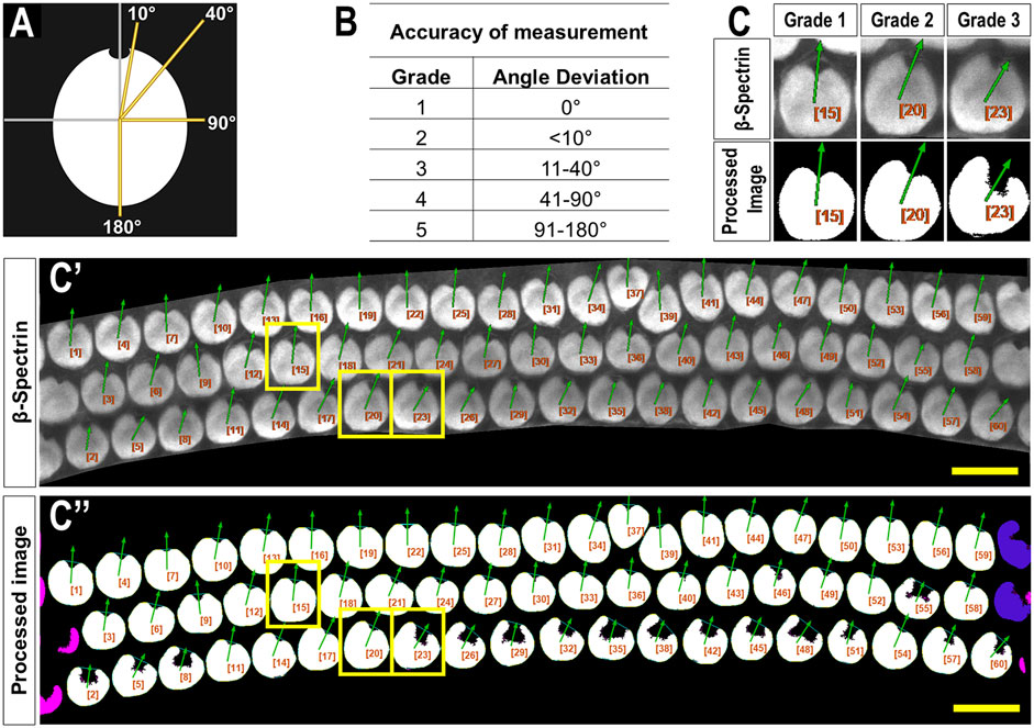
Both investigators used the following PCPA settings: remove noise of ≤500 pixels or fewer, exclude chunks ≤10 pixels from the image border, apply the Plastic Wrap function, and separate doublets when chunks measured ∼2 times wider than they were tall. Investigators differed on the following settings: investigator one ignored caves ≤3 pixels and selected the largest cave as the directional point of interest. Investigator two ignored caves of ≤15 pixels and selected the northmost cave as the directional point of interest. Angle measurements were set on a counter-clockwise 0°–360° scale where 90° pointed north. A third investigator was provided the original images with an overlay of arrows drawn by PCPA. This investigator assigned each analyzed cell an accuracy score from 1 to 5 (1 = perfect measurement; 2 = <10° deviation; 3 = 11°–40° deviation; 4 = 41°–90° deviation; 5 = 91°–180° deviation; Figure 2).

Figure 2. Criteria used to evaluate PCPA angle measurement accuracy. (A) A blinded investigator was instructed to consider an accurate planar cell polarity measurement as a ray originating from the center of mass of a cell and extending through the center of the fonticulus. The investigator then evaluated the directional arrow drawn by PCPA and assigned each cell an accuracy score from one to five using the grades shown in the table in (B) and the schematic from (A) as a reference. (C) Magnified view of example cells taken from a representative cochlear image (C’) showing matching angle accuracy scores of 1,2, and 3 which were derived by PCPA after incomplete thresholding of the cochlear hair cells (C’’). Yellow boxes indicate the cells chosen for magnification. Size excluded cells are pseudo-colored pink, and border excluded cells are pseudo-colored blue. Scores beyond three were not reported for any of the images analyzed (scale bars = 10 µm).

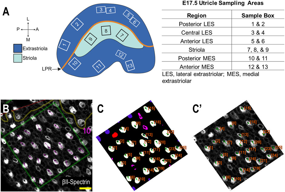
In order to systematically survey hair cells across different anatomical regions of the utricle, sample boxes (500 × 500 pixels) within the following regions were drawn (Figure 3): posterior lateral extrastriolar (boxes 1 and 2), central lateral extrastriolar (boxes 3 and 4), anterior lateral extrastriolar (boxes 5 and 6), striola (boxes 7, 8, and 9), posterior medial extrastriolar (boxes 10 and 11), and anterior medial extrastriolar (boxes 12 and 13). Boxes were oriented perpendicular to the line of polarity reversal as drawn onto the image by one of two investigators charged with manual angle measurements. To manually measure planar cell polarity, investigators were instructed to bisect the cuticular plate and continue through the center of the fonticulus, using the arrow tool in Fiji.

Figure 3. Performance of PCPA against manual PCP measurements for the E17.5 utricle (Panel (A) created with BioRender.com). (A) Example of regional sampling for E17.5 utricle analysis. Boxes were generally aligned according to the line of polarity reversal (LPR). (B) Example of manually collected PCP measurements from box 10 region of an E17.5 utricle. (C) The image from (B) was preprocessed, made binary, and analyzed using PCPA. The PCPA angle measurements show high agreement with manual measurements in (B). (C’) Directional arrows (green) and cell ID overlays (orange) were overlaid on the original micrograph. (scale bars = 10 µm).

Automated angle measurements were collected by a third investigator who was provided the same utricle images used for manual angle measurements described above. After image preprocessing (described above), binary images were analyzed by PCPA using the following settings: remove noise of ≤500 pixels or fewer, exclude chunks ≤10 pixels from the image border, apply the Plastic Wrap function, separate doublets when chunks measured 1.5 times wider than they were tall, ignore caves of ≤15 pixels and select the largest cave as the directional point of interest. Angle measurements were set on a counter-clockwise 0°–360° scale where 90° pointed north.

Images of murine radial glia from Mirzadeh et al. (Mirzadeh et al., 2010) and images of ependymal cells taken from Boutin et al. (Boutin et al., 2014) underwent channel splitting (Image > Color > Split Channels), and each channel image was converted to 8-bit grayscale (“Image > Type > 8-bit”). Each channel image then underwent manual thresholding (“Image > Adjust > Threshold”). Noise removal (“Process > Noise > Remove Outliers; ” radius = between 2–10 pixels; threshold = 50) was applied to each image and for the ependymal cells an additional binary erode step was taken (“Process > Binary > Erode”). Image channels were then re-merged (“Overlay > Add image … ”), and the LUT was inverted (“Image > Color > Invert LUTs”).

Images of Drosophila ommatidia taken from Koca et al. (Koca et al., 2022) were each duplicated (Image > Duplicate), then a manual threshold was applied to the duplicated image to leave only the cell junctions visible, the LUT was inverted so that the junctional borders would appear white rather than black, and Fiji’s “Process > Binary > Dilate and/or Erode” was used to connect the lines as much as possible while leaving empty space in the center of each ommatidium. This image was then added back to the original as a zero-transparent overlay (“Image > Overlay > Add Image … ; ” select “Zero Transparent”) and the image was flattened (“Image > Overlay > Flatten”). This image was then manually thresholded (“Image > Adjust > Threshold”) to isolate the rhabdomeres. The LUT was then inverted (“Image > Color > Invert LUTs”), and binary dilate (“Process > Binary > Dilate”) was applied until rhabdomeres touched to form a u- or h-shaped chunk. PCPA was then run on the images using Plastic Wrap and the selection for the largest cave.

Mean angles, resultant mean length (RML), circular variance, and circular standard deviation were calculated by PCPA using equations based on Fisher (Fisher, 1993) (equations provided in the user manual). All rose diagrams and descriptive statistics generated using PCPA were checked for accuracy against rose diagrams and descriptive statistics generated from the same data using the circular package (Agostinelli, C. and Lund, U. (2023). R package “circular”: Circular Statistics (version 0.5-0). URL https://CRAN.R-project.org/package=circular, n.d.) in R. Inter-rater reliability for angular measurements of utricle hair cells was tested using the SimplyAgree package in R (Caldwell, 2022). The mean of cell angle measurements from each image was paired between the manual blinded investigator and PCPA, and from these a concordance correlation coefficient and Bland-Altman limits of agreement were generated, again using the SimplyAgree package in R.

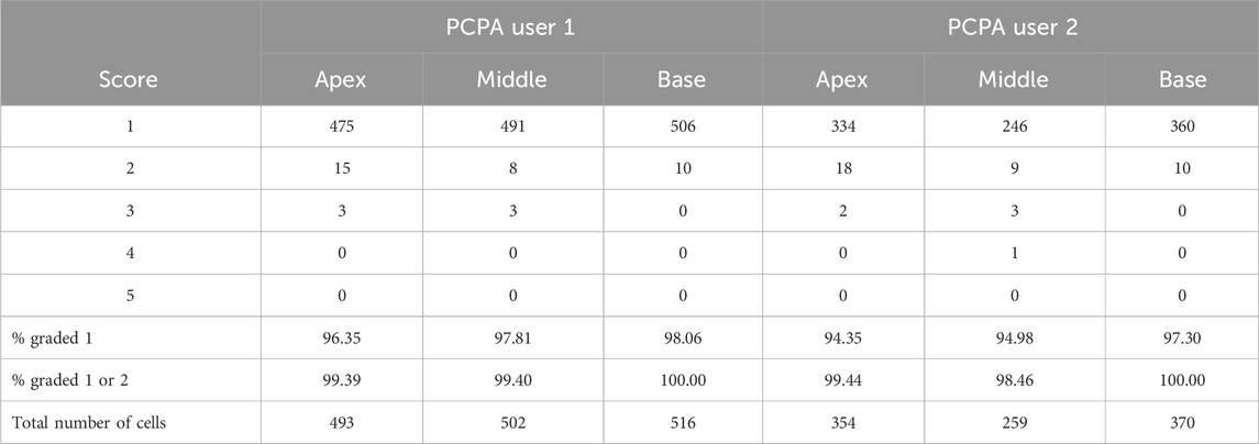
To test PCPA’s ability to count cells and calculate polarity we first tested PCPA on mouse cochlear hair cells. Two investigators were provided with 24 cochlear images from P4 mice (2 images per cochlear apex, middle, and base; n = 4 mice). Each investigator independently preprocessed the images and ran PCPA. Angle calculations from PCPA were rated for accuracy by a third investigator using a one to five agreement score (Figure 2) and overall accuracy scores per cochlear turn were calculated for each rater (Table 1). For cell counting, PCPA achieved 99.81% accuracy with PCPA being able to readily detect 1,538 out of 1,541 hair cells across the images analyzed. For PCP angle measurements, 96.35% (apex), 97.81% (middle), and 98.06% (base) of cells analyzed were scored as a one (perfect measurement). When cells scored one and two were combined—indicating cells that had <10° variation between PCPA measurements and idealized retrospective manual measurements—99.41% (apex), 98.93% (middle), and 100% (base) of cells analyzed by PCPA met this criterion. These data suggest that PCPA is able to accurately measure over 96% of βII-spectrin labeled hair cells in a data set, with perfect precision as determined by a human rater, and this metric jumps to over 98% when allowing for a <10° deviation from ideal.

Table 1. Accuracy of PCPA angle measurements from P4 cochleae.

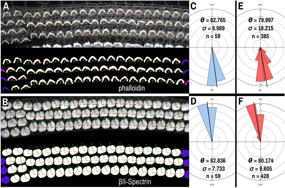
Though βII-spectrin staining of the apical surfaces of hair cells presents as rather ideal circular chunks and caves, we tested whether PCPA could be used with another commonly used fluorescent label: phalloidin. Phalloidin binds to the F-actin rich hair cell stereocilia and the vertex of the “V” shape of the stereocilia bundles in cochlear outer hair cells has been used to assess cell polarity (Montcouquiol et al., 2003; Jones and Chen, 2008; Copley et al., 2013). After preprocessing and making the phalloidin images binary, application of the Plastic Wrap function allows PCPA to bridge the distance between the legs of the phalloidin positive bundle, and thus create a large cave. Selecting the largest cave as the directional point of interest causes PCPA to calculate polarity angles that were directionally opposite to measurements using the fonticulus as the directional point of interest (Figures 4A,B). We compared PCP measurements obtained from βII-spectrin to the reversed values of those obtained from phalloidin on the same samples (acquired at the same time as multi-channel images that had high SNR for both phalloidin and βII-spectrin). When the phalloidin imaging was optimal, PCPA was able to measure the same number of outer hair cells with similar angle results (Figures 4A–C). Across eight images of outer hair cells from N = 3 mice PCPA results indicated that the phalloidin approach resulted in fewer hair cells measured (n = 385) compared to the βII-spectrin approach (n = 428). Mean angle measurements remained similar, with a measurement of 79.997° (±18.215°) for the phalloidin staining approach and a mean angle measurement of 80.174° (±9.605°) for the βII-spectrin staining approach, though the variability was greater for the phalloidin images (Figures 4E,F). These results show the capability of PCPA to perform automated analysis of cell polarizations and to obtain reliable mean angle measurements from multiple markers. Although the data suggest that using βII-spectrin staining results in slightly greater numbers of cells being measured and decreased variability compared to phalloidin, these discrepancies likely reflect the previously reported lesser reliability of phalloidin as compared to spectrin, pericentrin, or other antibody labeling that clearly demarcate the position of the fonticulus (or kinocilium) (Deans et al., 2007; Yin et al., 2012).

Figure 4. PCPA analysis of cochlear outer hair cells labeled with AlexaFluor488 conjugated phalloidin. Phalloidin (A) and βII-spectrin (B) labeled outer hair cells were imaged in different channels of the same P4 mouse cochleae, then the channels were separated and thresholded for PCPA analysis (thresholded outputs shown in the bottom half of each panel). In both (A) and (B), size excluded cells are pseudo-colored pink and border excluded cells are pseudo-colored blue. (C) PCPA analysis of the image in (A) resulted in angle measurements collected from n = 59 outer hair cells with a mean angle (θ) of 82.765° and a standard deviation (σ) of 9.989°. (D) PCPA analysis of the βII-spectrin channel from this same cochlear region also measured angles from n = 59 outer hair cells with a resultant mean angle of 82.836° and a standard deviation of 7.733°. (E) The analysis was expanded to eight images of phalloidin-labeled cochlear outer hair cells; PCPA was able to measure n = 385 cells and arrive at a mean angle of 79.997° (σ = 18.215). (F) PCPA analysis of βII-spectrin labeled cells from the same eight samples resulted in angles being measured from n = 428 outer hair cells with a mean angle of 80.174° (σ = 9.605). Thus, PCPA is able to measure planar cell polarity using images of phalloidin labeled cochlear outer hair cells. However, while the resultant mean angles in (E) and (F) were highly similar, the number of cells measured was greater when βII-spectrin labeling was used, and the variability of the measurements was reduced as compared to the phalloidin data (F) vs (E). (scale bars = 10 µm).

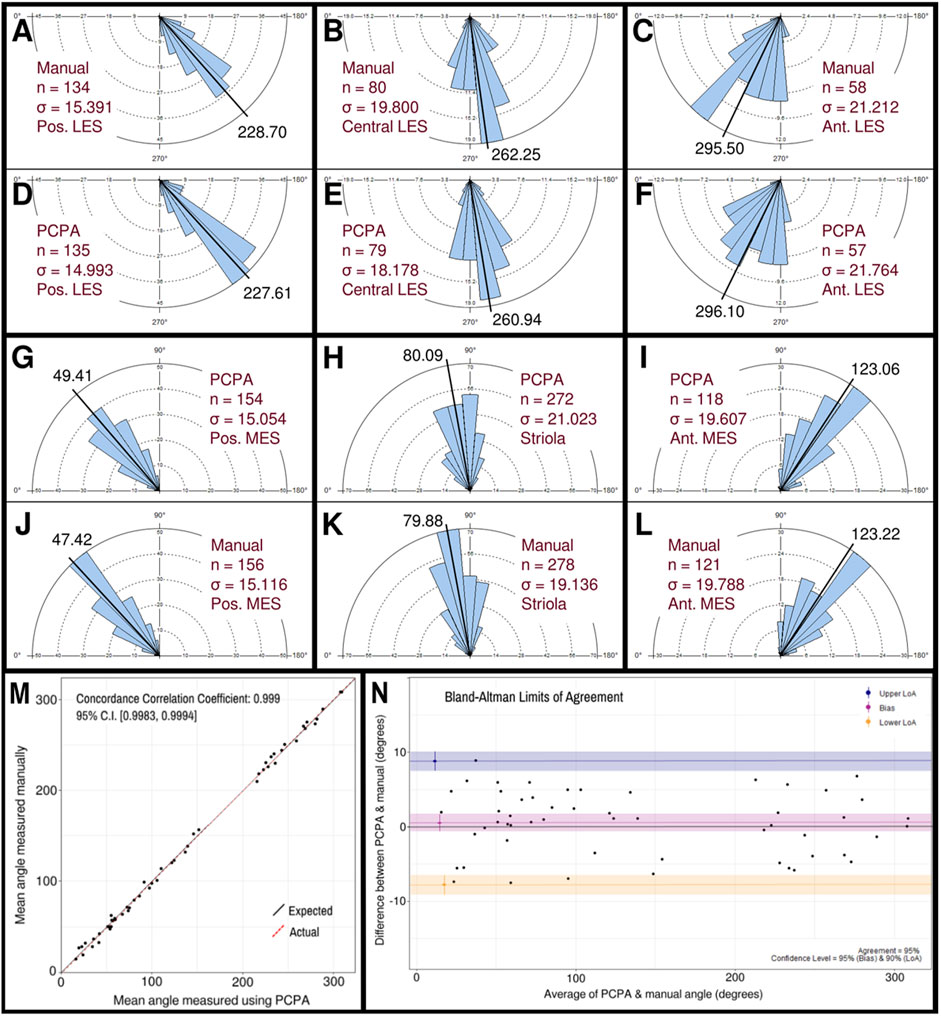
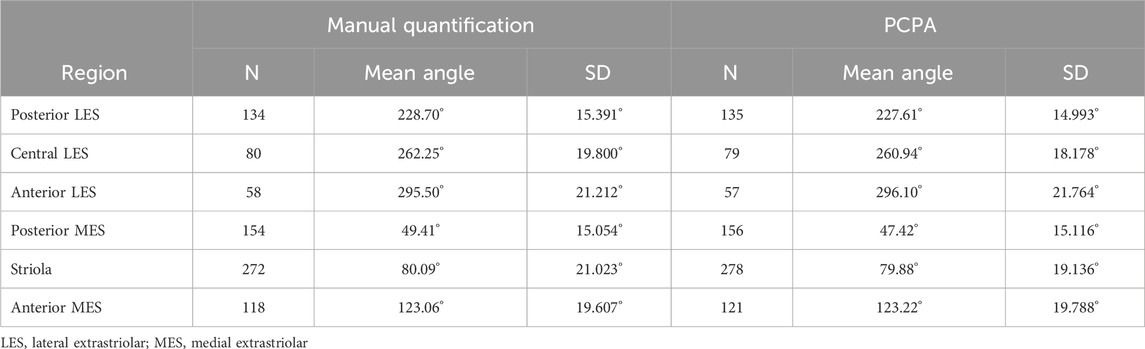
The performance of PCPA was next tested on E17.5 utricle images which had been collected as control samples for a separate project in the laboratory. As these images were collected prior to the development of PCPA, the image acquisition parameters were not optimized to maximize βII-Spectrin fluorescent intensity, thus making them ideal “real-world” examples for testing. Sample boxes (500 × 500 pixels) were taken from posterior lateral extrastriolar, central lateral extrastriolar, anterior lateral extrastriolar, striola, posterior medial extrastriolar, and anterior medial extrastriolar regions (Figure 3). Cell angle measurements were collected manually by investigators instructed to bisect the hair cell apical surface and the fonticulus using the Fiji arrow tool and to record the angle as measured by Fiji. Another investigator preprocessed the images, converted them to binary, and used PCPA to measure the angles of the same cells that were quantified manually. Since the manual measurements did not indicate which angle measurement corresponded to which individual cell in any given image, the degree of agreement between the two data sets was assessed using the mean angle value from each image or image-pair as shown in Figure 5A–5L. Sample size was thus n = 54 mean angle measurements from 5 separate embryos from two distinct litters and the data are reported in Table 2. Calculation of the concordance correlation coefficient (CCC) showed a high level of agreement between the manually quantified data and PCPA quantified data (CCC = 0.999; 95% C.I. [0.9983, 0.9994]) (Figure 5M). Calculation of the Bland-Altman limits of agreement suggest minimal bias for the PCPA measurements as compared to manual measures, with a value of 0.482° (95% C.I. [−0.676, 1.64]). The limits of agreement (LoA) were calculated at a 95% agreement level with the lower LoA at −7.833 (90% C.I [−9.143, −6.523]) and the upper LoA at 8.798 (90% C.I. [7.487, 10.108]). As shown in Figure 5N, the Bland-Altman analysis suggests that nearly all PCPA measured mean angles from similar images could be expected to fall between −8 and +9 degrees of manually obtained mean angle measures.

Figure 5. Manual vs PCPA obtained angle measurements of βII-spectrin labeled hair cells in E17.5 mouse utricles. Manual measurements of hair cell orientations with respect to the LPR were taken as described in the manuscript main text and in Figure 4. A Rose diagram was plotted using PCPA (or stand-alone Rose Diagram plug-in) to visualize the results from each region investigated. For each region, the mean angle is represented by a black line and the exact value reported in black text. The number of cells in each region that were measured (n) and the circular variance in degrees (σ) is also provided. Manually obtained data for the LES are presented in the outer rows and can be directly compared to PCPA data in the central rows such that manual vs. PCPA for the posterior LES region (A vs. D), central LES (B vs. E), and anterior LES (C vs. F) are readily visualizable in the top two rows and manual vs. PCPA data for the posterior MES (J vs. G), striola (K vs. H) and anterior MES (L vs. I) are visualizable in the fourth and third rows. (M) Inter-rater reliability was assessed for manual vs. PCPA measurements by plotting the mean angles for each image as a function of the PCPA value along the x-axis and the manual value along the y-axis, which, in the case of perfect agreement would yield a bisecting diagonal line (“Expected” shown in black). A line of best fit for the actual values (“Actual” shown in red) was plotted and the concordance correlation coefficient calculated as 0.999 (where a value of one would indicate absolute agreement for all values). (N) A Bland-Altman plot was generated again using the mean angle values from each image analyzed and upper and lower limits of agreement were calculated. The red line suggests a very small value for bias (<0.5°) with a confidence interval (pink) that lies on both the positive and negative sides of zero. The blue and yellow lines represent the upper and lower limits of agreement, respectively, at a confidence level of 95%.

Table 2. Utricle measurements: Manual quantification vs PCPA.

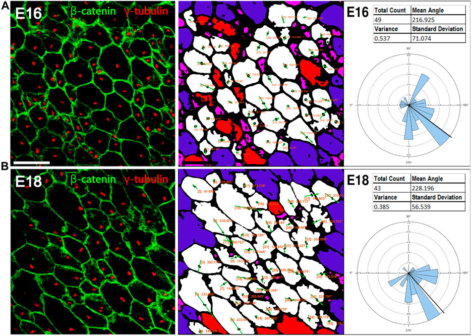
Because planar cell polarity is found in a variety of tissues outside of the inner ear, we sought to test the PCPA plug-in on other image types including those using different labels, as well as samples from both wild-type animals and PCP mutants. To accomplish this, we collected images from several peer reviewed publications, preprocessed the images, ran PCPA, then compared PCPA’s results to published results. We first tested PCPA using images of radial glial cells from E16 and E18 mice from Mirzadeh et al. (Mirzadeh et al., 2010) In that report, cell junctions were labeled with an anti-beta-catenin antibody and primary cilia were labeled using an anti-γ-tubulin antibody (red and green, respectively, in the published figures). PCPA results (Figure 6) demonstrate the effective measurement of cell polarity with a decrease in variability in polarization evident from E16 (SD = 71.1) to E18 (SD = 56.5), consistent with the increasing alignment of the cells with developmental progression.

Figure 6. PCPA effectively measures radial glial progenitor cell orientations. Leftmost image in (A) and the leftmost image in (B) were reproduced from Mirzadeh et al. (Mirzadeh et al., 2010) (licensed under CC-BY-NC-SA 3.0). Cell junction labeling with anti-β-catenin (green) and labeling of primary cilia with anti-γ-tubulin immunolabeling (red) were used in this study to assess PCP in radial glial progenitors from (A) E16 and (B) E18 mouse embryos. PCPA analysis of these images correctly defines the predominant angle as toward the bottom left corner of the images (216°–228°) and demonstrates reduced variability as the alignment of cell direction becomes more consolidated during normal development from E16-E18.

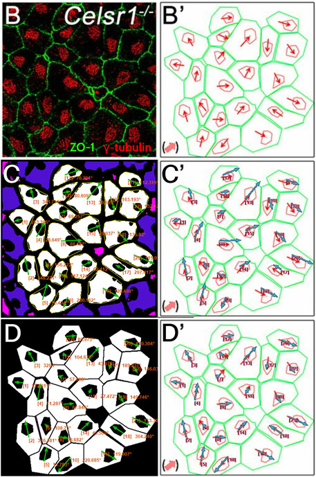
Next, we tested PCPA’s performance on ependymal cell orientation using images from wildtype and Celsr1 knockout mice (Supplementary Figure S5; Figure 7). In the original report, Boutin et al. (Boutin et al., 2014) manually traced the perimeter of each ependymal cell using anti-ZO1 labeled cell junctions, then traced the perimeter of the cell’s γ-tubulin positive cilia patch. They then determined cell directionality utilizing a custom MATLAB script that, similar to PCPA’s approach, calculated angles based on the center of mass of the traced perimeter of the cilia patch in relation to the center of mass of the traced perimeter of the cell junction. We compared cell orientation results reported in Boutin et al. (Boutin et al., 2014) to those generated by PCPA and found that PCPA was able to replicate Boutin et al.’s (Boutin et al., 2014) angle orientations with a high degree of agreement (Figure 7; Supplementary Figure S5). One noted exception occurred in the Celsr1 knockout sample where one cell’s PCPA-derived angle projection was nearly 180° opposite to the published data (cell number 6; Figure 7C, C’). Because Boutin et al.’s (Boutin et al., 2014) preprocessing workflow required an investigator to manually trace the cell perimeter, we speculated that the difference between PCPA and the published result could be due to the tracing process. Indeed, when we re-ran PCPA using Boutin et al.’s (Boutin et al., 2014) tracings (Figure 7D−7D′), the directional disagreement for cell number six was resolved.

Figure 7. PCPA recapitulates angle measurements from ependymal cells in a Celsr1 knockout mouse model. Panels (B) and (B’) are replicated from Figure 4B,B’ of Boutin et al. (Boutin et al., 2014) (reproduced under the PNAS license to publish agreement). (B) A confocal image of Celsr1−/− mouse ependymal cells labeled with antibodies against ZO-1 (green) and γ-tubulin (red). (B’) Manual tracings (green and red) of the cells in (B) with overlaid angle measurement arrows (red), as originally shown in Boutin et al. (Boutin et al., 2014). (C) Annotated output of image (B) after preprocessing and data collection with PCPA. The annotated output shows Plastic Wrap (yellow), edge excluded chunks (blue), size excluded chunks (pink), cell ID number with angle measurement (orange text), and vector arrows (green). (C’) Arrows from PCPA analysis (blue) are overlaid onto the image from (B’) to show the high level of agreement between PCPA and Boutin et al.’s (Boutin et al., 2014) published data. Only one cell exhibited stark disagreement (cell #6), where the angle measured by PCPA appears nearly 180° opposite the published result. (D) Since Boutin et al. (Boutin et al., 2014) measured manual tracings of the original image, we preprocessed the manual tracing image and analyzed this with PCPA. (D’) Overlaid arrows from PCPA analysis (blue) using the manual tracings show complete agreement with those in the original published work, suggesting any deviations in (C and C’) are likely the result of differences in pre-preprocessing approaches (i.e., the use of a thresholded image versus manual tracings).

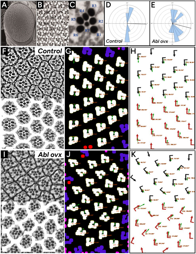
Finally, we compared PCPA’s performance on brightfield images of osmium (OsO4) fixed Drosophila ommatidia from Koca et al. (Koca et al., 2022). Analysis of Drosophila ommatidia required a slight alteration to the preprocessing steps established above for PCPA to isolate the rhabdomeres in the photoreceptor cells (see methods section for details). PCPA produced angle orientations comparable to the manually obtained orientations collected by Koca et al. (Koca et al., 2022) for ommatidia from WT (Figures 8F–H) and Abl-overexpression mutants (Figures 8I–K). PCPA measurements from these images have near complete agreement to the published results (Figures 8H,K), and demonstrate the ability of PCPA to detect disrupted cell polarization in PCP mutants (Figure 8D vs. 8E and 8H vs. 8K). All together, these results show that PCPA has the ability to collect PCP angle measurements from a variety of diverse cell and tissue types collected with various staining and imaging parameters, and works in models with normal or disrupted PCP.

Figure 8. PCPA replicates angle measurements of wildtype and Abl overexpressing Drosophila ommatidia. Panels (A) and (B) were reproduced from Figures 1A,C from Tomlinson et al. (Tomlinson et al., 2011) (licensed under CC-BY 4.0). Panels (E), (G), (H), and (J) were adapted from Figures 2A,B from Koca et al. (Koca et al., 2022) (licensed under CC-BY-NC-ND 4.0). (A) A lower magnification scanning electron microscopy image of the eye of the fruit fly and (B) an image taken under higher magnification with a light microscope after sectioning highlights the seven readily visible rhabdomeres from which PCP can be determined. (C) A rose diagram generated by PCPA of wildtype/control Drosophila ommatidia shown in panels (F–H) shows that the ommatidia are well aligned along the vertical axis. (D) A rose diagram generated by PCPA of ommatidia in Abl overexpressing Drosophila shown in panels (I–K) shows disruption of the vertical alignment. Images for analysis were copied from Koca et al. (Koca et al., 2022). (F) Wildtype/control ommatidia (top) with overlay mask (bottom) created during PCPA preprocessing to mask ommatidial junctions. (G) PCPA annotated output showing Plastic Wrap (yellow), edge excluded chunks (blue), size excluded chunks (pink), unmeasurable chunks (red), the resulting angle measurements (orange text), and vector arrows (green). (H) The PCPA output overlay (green arrows) was added to the measurements presented in Koca et al. (Koca et al., 2022) (red arrows) to show the general agreement between PCPA and published measurements. (I) Abl overexpressing ommatidia (top) with overlay mask (bottom) created during PCPA preprocessing to mask ommatidial junctions. (J) PCPA annotated output showing Plastic Wrap (yellow), edge excluded chunks (blue), size excluded chunks (pink), unmeasurable chunks (red), the cell ID number with resulting angle measurements (orange text), and vector arrows (green). (K) The PCPA output overlay (green arrows) was added to the measurements presented in Koca et al. (Koca et al., 2022) (red arrows) to show the general agreement between PCPA and published measurements for the more disorganized ommatidia of the Abl overexpression mutant.