1 Introduction

Cervical cancer is currently the most common cancer of the female reproductive system globally, with approximately 30%–40% of cervical cancers occurring in young women (1). Patients with early-stage cervical cancer who have high pathological risk factors for recurrence after radical hysterectomy need adjuvant radiotherapy or chemotherapy. The dose of conventional postoperative radiotherapy for cervical cancer is 4,500 cGy or greater, but the ovaries are sensitive to radiation. Some studies have shown that doses above 400 cGy can lead to permanent ovarian failure, early menopause, some menopausal syndromes, etc. (2). As a result, young patients often undergo ovarian transposition during a radical hysterectomy to move their ovaries out of the pelvic region that is potentially the field of radiation, which can significantly reduce the dose to the ovaries. However, current data show that only approximately 50% of transposed ovaries retain their function, even if the ovaries have been removed from the potential radiation field (3–5). The ovarian survival rate still needs to be improved. Studies have shown that the maintenance of ovarian endocrine function after radiotherapy in cervical cancer patients is directly related to ovarian dose (6, 7), which is closely associated with the location of the transposed ovaries. Therefore, during ovarian transposition, it is particularly important to determine the appropriate location for ovarian placement and ensure that the dose of the ovaries in postoperative adjuvant radiotherapy is below safe limits.

Current research on the location of the transposed ovary is mainly based on statistical methods (8–10). By analyzing data from 150 patients who had undergone ovarian transposition and received postoperative radiotherapy, LV et al. (8) plotted the operating characteristic curve (ROC) of ovarian position versus the dose received and concluded that moving the ovaries above 1.12 cm in the iliac crest plane enabled the dose to be controlled below the safety limit. J Toman et al. (9) monitored the ovarian endocrine function following pelvic external beam radiation with the ovaries at various transposition locations and discovered that the ovaries were safe beyond 2.5 cm of the radiation field edge. Nevertheless, each patient’s anatomy and pathology staging affect the size of the target area in radiation. Even if the ovaries are all located 2.5 cm from the radiation field edge for various people, the radiation dose may differ significantly. As a result, the findings from earlier studies were not patient-specific and might not be appropriate for all individuals.

Researchers have recently utilized deep learning to predict the dose distribution for several cancer types, including prostate, rectal, and cervical cancers (11–13). The U-net and several U-net-like models are typically the foundation of current experiments employing deep learning for the dose prediction (14–16). However, it has been documented that due to the physical characteristics of volumetric modulated arc therapy (VMAT) dose, traditional U-Net models often do not predict the VMAT dose distribution well, especially in low dose regions (17, 18). To improve the ability of neural network models to predict VMAT dose distribution, we propose a novel progressive refinement attention model with deep supervised strategy and weighting self-attention architecture, which can improve the generalization and robustness of the model. Then, the model is applied to the prediction for the dose distribution. The predicted dose distribution can be visualized on preoperative computed tomography (CT), which then can be used to determine the location of the ovary during ovarian transposition surgery so that the dose of the ovary in postoperative radiotherapy is below the safety limit. By using a neural network model that exploits the characteristic relationship between patient anatomy and dose distribution, the dose distribution can be predicted more accurately based on the unique anatomy of each patient, and thus the appropriate transposed ovarian location can be predicted.

2 Materials and methods

In this study, a new progressive refinement attention model, PRT-Net, was used to predict the dose distribution. The preoperative CT slices, organs at risk (OARs), and PTVs were used as the input of the model. The dose distribution of the planning CT was mapped to the preoperative CT and used as the output of the model. Note that the planning CT is the CT taken after ovarian transposition, namely, postoperative CT. This output of the model combining the dose distribution with preoperative CT will provide a low dose region that will be the range for the ovarian transposition. The surgeons can then determine the safe location of ovary prior to surgery based on clinical knowledge within this range. A flow chart showing the process of this study is demonstrated in Figure 1.

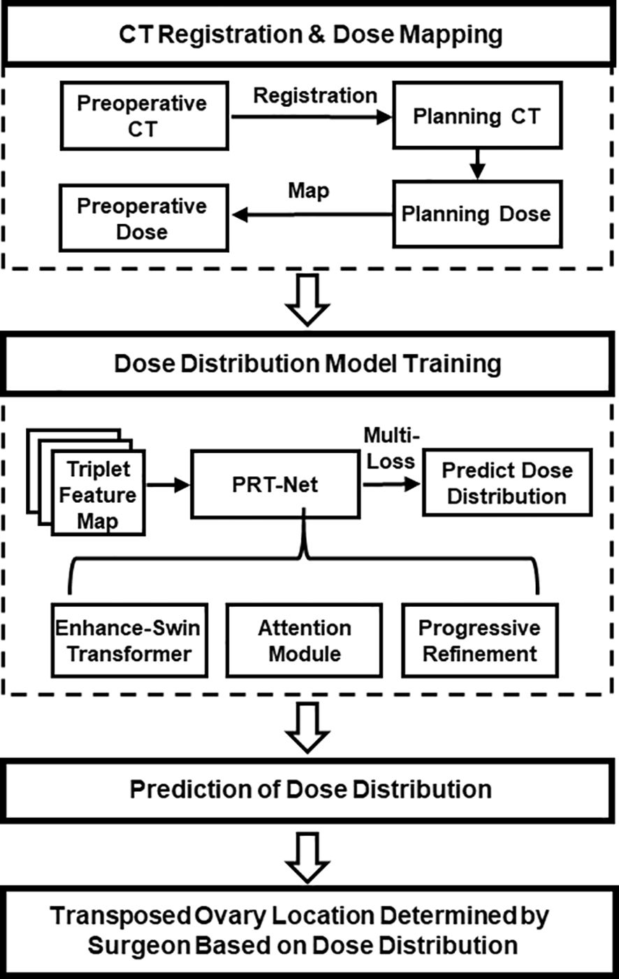
Figure 1 Overall workflow of the study.

2.1 Patients and treatment planning

In this study, the clinical data of 104 patients (69 cases were randomly selected as training data, 22 as validation data, and the remaining 13 as test data) with cervical cancer who received postoperative radiotherapy in Hubei Cancer Hospital, Wuhan, China, were collected. Prior to radical hysterectomy, preoperative CT was obtained using SOMATOM Definition AS+ (Siemens, Berlin, Germany), with a slice thickness of 5 mm. The patients were immobilized in the supine position by vacuum cushions. Planning CTs were acquired with a Brilliance CT (Big Bore, Philips, Cleveland, OH, USA), and the slice thickness was also 5 mm.

The clinical target volume (CTV) and OARs including bladder, rectum, small intestine, bilateral femoral heads, marrow, and spinal cord were delineated by an attending oncologist. The prescription was 45 Gy in 25 fractions (1.8 Gy per fraction) to the planning target volume (PTV) generated with 0.5 cm uniform expansion from the CTV. All VMAT plans are using two full arcs with 6-MV energy, designed in the Monaco treatment planning system (TPS) (version 5.11.01, Elekta, Stockholm, Sweden) with the Monte Carlo algorithm for an Infinity accelerator (Elekta, Stockholm, Sweden).

According to ICRU (International Commission on Radiation Units and Measurements) Report 83, D95% of the PTV is greater than the prescribed dose, D2% is less than 110% of the prescribed dose, and D98% is greater than 95% of the prescribed dose. For the evaluation of OAR for cervical cancer, reference was made to the RTOG (Radiation Therapy Oncology Group) Report 0418 and the actual situation of our institution. The corresponding evaluation criteria are as follows: V30<50%, V40<40%, V45<35% for bladder, V30<60%, V40<55% for rectum, V30<15% for femur head, and Dmax<45 Gy for spinal cord.

2.2 Dose alignment

The dose from the planning CT needs to be mapped to the preoperative CT in order to show the dose distribution on the preoperative CT, allowing surgeons to quickly determine the safe location of the transposed ovarian before the surgery. The image processing software MIM (version 6.8.7, MIM Software Inc., USA) was used to achieve image registration between preoperative and planning CT of the same patient using rigid alignment. Considering that the uterus, lymph nodes, and other structures are removed during radical hysterectomy for cervical cancer, the OARs will be greatly deformed between the preoperative CT and the planning CT. Therefore, the contours of targets and OARs of the pre-operative CT of each patient were manually revised by the radiation oncologist.

2.3 Data preprocessing

Raw CT pixel values were converted to Hounsfield units (HU) on a scale between -1,000 and +400. Each OAR and PTV contours were filled with 0 (background) and 1 (foreground) to transform into the binary mask. The PTV, bladder, femoral head left, femoral head right, kidney left, kidney right, marrow, rectum, spinal cord, and body were chosen as the relevant structures for VMAT dose prediction. The dose distribution was resampled to a voxel size of 2.5 × 2.5 × 5.0 mm by using single linear interpolation. In addition, the original image feature matrix was resampled to 512 × 512 pixels using the zero filling method.

To allow our neural network to learn the volumetric features, training was performed using image triplets input (19), which combines three consecutive 2D CT slices and their corresponding binary segmentation masks. Each 2D CT slice and a binary segmentation mask are combined into a superimposed feature map with 11 channels, denoted as x∈R11×512×512, then concatenated with three sets of spatially continuous superposition feature maps together along the channel dimension to form a final triplet feature map with 33 channels, denoted as x∈R33×512×512.

2.4 Quantitative dose prediction evaluation

To quantitatively evaluate the accuracy of the network model, we compared the dose prediction results of PRT-Net with three other neural network models [U-Net (20), U-net++ (21), and DeepLab-V3-plus (22)]. The evaluation metrics include mean absolute error (MAE), mean squared error (MSE), root mean square error (RMSE), absolute differences of dosimetric parameters between the real and predicted dose in the OARs and PTV, the dose–volume histogram (DVH), gamma index, and the isodose volume DSC, including the 4-, 10-, 15-, and 20-Gy isodose regions. All evaluation indexes are based on body contour as a mask, with the following formula:

Gamma index passing criteria was 3%/2 mm, and only the dose exceeding 10% of the maximum dose was calculated. In addition, areas outside the body were not included in the gamma index calculation.

The DSC of the isodose volume was evaluated in the 3D dose distribution. The DSC calculates the overlapping results of two different volumes based on Equation 1:

where A is the real isodose volume and B is the predicted isodose volume.

2.5 Implementation details

For training neural networks, Adam with a weight decay of 0.0001 was utilized to optimize network parameters, with the initial learning rate set to 0.0001. The batch size was set to 16, and the epoch size was set to 100. The neural network using PyTorch was implemented, and experiments were performed on a small NVIDIA RTX3090Ti workstation equipped with 24 GB of RAM.

3 Network architecture

We proposed a new progressive refinement attention model, Swin-Refinement-Attention (PRT-Net), based on the Swin-Transformer architecture (23), as shown in Figure 2. The model uses an efficient encoding module to extract superimposed feature map information, an attention module (24) to assign feature weights over space and channels and a decoder to gradually generate dose distribution from low- to high-scale resolution.

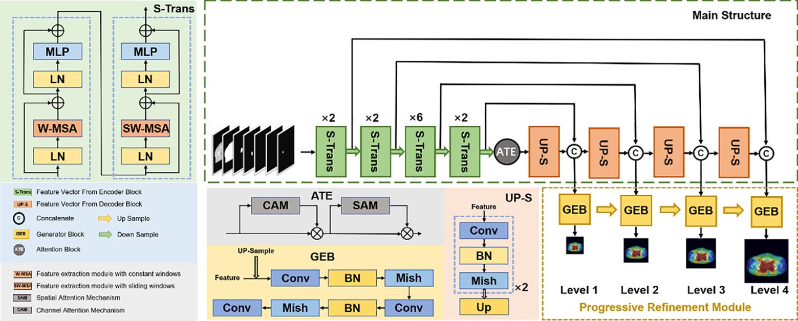
Figure 2 Schematic diagram of the proposed PRT-Net architecture.

3.1 Encoding module

Considering that the traditional convolutional neural network (CNN) encoding architecture is unable to obtain global information at local locations and that the receptive field mechanism is prone to lose detailed semantic features, we adopted an encoding architecture based on the transformer, as shown in Figure 2. The encoding module consists of four enhanced Swin-Transformer encoders, each containing two mutually independent feature extraction modules (the constant window and the shifted window). Before feeding the input features into the enhanced Swin-Transformer layer, several pre-processing operations need to be performed on the raw feature maps. First, the original features x∈RC×H×W were split into N N=HP×WP tokenization x∈RC×P×P of the same size by the window splitting algorithm, where P is the patch size and C is the channel dimension. Then, to match the input of the enhanced Swin-Transformer layer, the linear projection function was used to convert the three-dimensional image patches into a two-dimensional embedding sequence xe∈RN×ce, where Ce represents the dimensionality of each embedding sequence. Finally, the generated embedding sequences were added with the prior position parameters to acquire the output sequence xp∈RN×ce, which was fed directly into the enhanced Swin-Transformer layer.

Distinct from the traditional Swin-Transformer algorithm with a multi-headed self-attention mechanism (25), we adopted the multi-head-enhanced self-attention (enhanced multi-headed self-attention mechanism) architecture. First, three learnable matrixes (the query matrix WQ∈RCe×dk, the key matrix WK∈RCe×dkand the value matrix WV∈RCe×dv, where dk=dv=Ceh, h represents an independent self-attention layer) with the output of the previous enhanced Swin-Transformer layer or input layer were used to calculate three sequence vectors (the query vector Q, the key vector K, and the value vector V), as shown in Equation 2. Then, the learnable weights matrix Wα∈Rdk×N was utilized to perform an enhanced self-attentive calculation on the query vector and the key vector to obtain the attention score, which was passed through the softmax activation function to acquire the normalized score, and then multiplied by each value vector to get the output vector SA(xl), as shown in Equation 3.

Multiple head cascades W−MSAxl for calculating the self-attention scores in different subspaces were generated to capture the correlation between different subspaces of the sequence, as shown in Equation 4, W−MSA denotes the enhanced self-attention algorithm with constant window, and then xl+1 was obtained by summing with the original high-dimensional spatial features using the residual mechanism, as shown in Equation 5, with LN denoting layer normalization. Ultimately, the output of the constant window-based feature extraction module can be obtained by Equation 6; MLP denotes multi-layer perceptron.

W−MSAxl= Concat SA(xl)1....SA(xl)h(4)x^l+1=xl+1+MLPLN(xl+1)(6)

The shift window feature extraction module SW−MSA was obtained by adding the window shift algorithm based on the W−MSA module. The cross-window connection introduced in SW−MSA while ensuring efficient computation of non-overlapping windows can fuse the feature information extracted from different windows and improve the model ability. The SW−MSA module employed window configurations distinguished from the regular window division of the W−MSA module, and SW−MSA module adopted shifting P2,P2 pixels relative to the top left pixel point as the new window. Ultimately, the output of the SW−MSA module can be obtained by Equation 7.

xl+2=SW−MSALN(x^l+1)+x^l+1+MLPLN(SW−MSALN(x^l+1)+x^l+1)(7)3.2 Attention module

To further improve the feature representation, we employed a lightweight convolutional attention operator that inferred attentional concentration regions along two specific and mutually independent dimensions and adaptively optimized local features by applying different attention scores for channel information and spatial information, respectively. The channel attention weight operator is shown in Equation 8. The channel weight operator was multiplied with the input feature map xl+2 to obtain the channel enhancement feature map x^l+2, as shown in Equation 9. The spatial attention weight operator is shown in Equation 10. The spatial weight operator was multiplied with the channel-enhanced feature map x^l+2 to obtain the channel–space enhanced feature map xl+3, as shown in Equation 11. Finally, the channel–space enhanced feature map xl+3 was added to the input feature map xl+2 to obtain the output feature map x^l+3 of the attention module, as shown in Equation 12. Due to its smaller and lighter architecture, the convolutional attention operator can be seamlessly integrated into the network architecture while ignoring its cost to perform end-to-end training together with the neural network.

Mc(xl+2) =σ(MLP(AvgPoolC×1×1(xl+2))+MLP(MaxPoolC×1×1(xl+2)))(8)Ms(x^l+2)=σ(Conv7×7([AvgPool1×H×W(x^l+2);MaxPool1×H×W(x^l+2)]))(10)xl+3=Ms(x^l+2)⊗x^l+2(11)

In the equations above, σ is the activation function sigmod and MLP is multi-layer perceptron. AvgPoolC×1×1 and AvgPool1×H×W denote the global channel pooling and global spatial pooling, respectively. MaxPoolC×1×1 and MaxPool1×H×W denote maximum channel pooling and maximum spatial pooling, respectively. Conv7×7 represents the convolution with a kernel size of 7×7. ⊗ denotes element multiplication.

3.3 Decoding module

To recover efficient semantic expressions, a decoding module containing up-sampling was employed to gradually recover the feature space information. The up-sampling was performed by the bilinear interpolation operator (26) with a scale factor of 2. Each decoding module consists of two consecutive series (convolution, batch normalization, Mish activation function), with the integral expression shown in Equation 13 and the Mish expression shown in Equation 14. All the convolutional layers in the decoding module have kernel size of 3×3 and padding size of 1. The number of channels is 512, 256, 128, and 64, respectively. The decoder can decompress the encoded medical image feature information and generate the corresponding dose distribution map.

xl+4=[Mish]×2 up-sample (13)Mish(x)=x·tanhln1+ex(14)

For each decoding module, the scale resolution of the feature map increases by a factor of 2. The skip connection between encoding and decoding modules not only introduces spatial information but also alleviates the common gradient problem in deep learning.

3.4 Progressive refinement module

As shown in Figure 2, the progressive refinement (17) module contains four predictive branches pi to predict the dose distribution at different scale resolutions. Each prediction branch contains a generation module G to generate the dose distribution map φiG of size ni×ni. The generation module consists of two consecutive series (convolution, batch normalization, Mish activation function) with a scaling tuned convolution, as shown in Equation 15. To ensure constant output dimensionality, all convolutional layers have a convolutional kernel size of 3×3 and padding size of 1.

φiG=conv1×3×3[Mish]×2 (15)

The low-scale resolution dose distribution map φiG was fed to the higher-scale prediction branch after bilinear interpolation up-sampling operation with a scale factor of 2. Then, elementwise addition with the dose distribution map at high-scale resolution was used to obtain φi+1G, as shown in Equation 16.

3.5.3 Rank loss

The most direct assessment of the quality of the dose distribution is to measure the DVH, which usually uses the percentile of the dose distribution to determine the dose metric—for instance, D98 is the value of the 98th percentile in the dose distribution, which means that the sequential relation of dose values can reflect the dose distribution. Therefore, we proposed a rank-based loss function Lr to ensure the order between the dose values in the dose prediction pi to be close to the real criteria yi. Firstly, the pixel values in pi and yi were vectorized and sorted in ascending order to get the pixel distribution yi* of yi with the corresponding pixel index λindex, which was used to reconstruct the pi pixel vector in order to obtain pi*. Secondly, the order of adjacent pixel metrics in yi* and pi* is shown in Equations 20 and 21, respectively, where σ∈[1,mi−1].

ρ(pi*(σ),pi*(σ+1))=exp(pi*(σ+1)−pi*(σ))1+exp(pi*(σ+1)−pi*(σ))(20)ω(yi*(σ),yi*(σ+1))={1,yi*(σ+1)>yi*(σ)1/2,yi*(σ+1)=yi*(σ)0,yi*(σ+1)<yi*(σ)(21)

Finally, the negative log-likelihood was used to measure the rank loss of pi versus yi, as shown in Equation 22.

Lr=−12mi∑j=1mi−1[ω(yi*(σ),yi*(σ+1))·logρ(pi*(σ),pi*(σ+1))+(1−ω(yi*(σ),yi*(σ+1)))·(1−logρ(pi*(σ),pi*(σ+1)))](22)4 Result4.1 Global dose prediction

As shown in Table 1, all four network models were trained using three different loss function algorithms. As can be seen in the table, DeepLab-V3-plus was slightly superior to PRT-Net in the MAE results obtained by training using the Lm&Lp algorithm, while in the remaining MSE, MAE, and RMSE indices, PRT-Net was the smallest of the four models. PRT-Net showed the least difference between the prediction and real data in the four models.

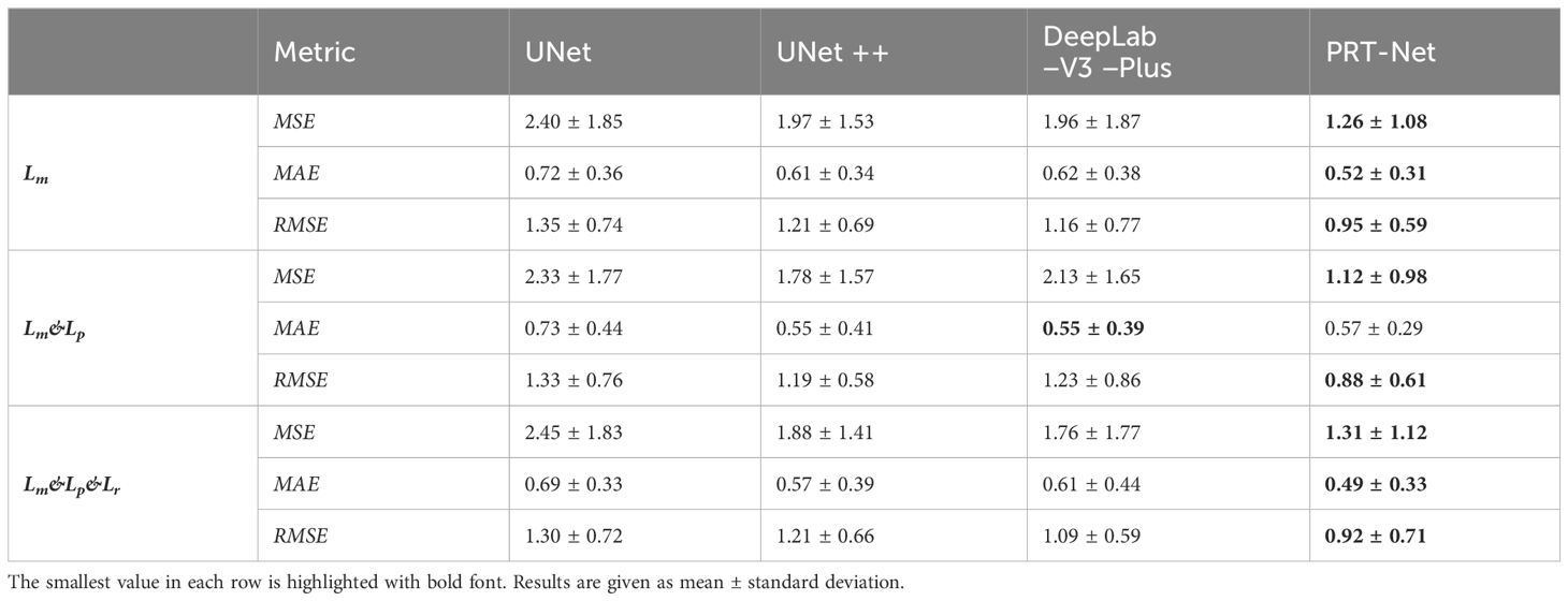
Table 1 MSE, MAE, and RMSE of the four models trained with three loss function algorithms.

We divided the remaining results into two parts, showing the comparison between the four network models and the comparison between the three loss function models.

4.1.1 Comparison between the four network models

The four network models were trained separately using the Lm loss function algorithm, and the results of each are shown below. Table 2 demonstrates the absolute differences between the dosimetric parameters predicted by the four neural network models and the real ones. As can be seen in the table, PRT-Net achieved optimal results for several metrics (PTV D2, bladder V30, V40, V45, rectum V30, V40, left femoral head, and right femoral head V30 had the smallest absolute errors among the four models). U-net++ also showed good results on several indicators (D95 and D98 for PTV and Dmax for the spinal cord). Figure 3 shows the dose distribution of three patients in the test cohort, including the real dose distribution and predicted outcomes in four models. PRT-Net is the closest to the real dose distribution in predicting the high dose range and the low dose range by comparing the predictions of the four models. Figure 4 shows the DVH curves predicted by the four network models. The OARs and PTV curves show that the DVH curves predicted by PRT-Net are the closest to the real curve in the four models, especially the PTV curves. Figure 5 shows the results of the 2D gamma analysis with 3%/2 mm criteria. This suggests that the U-net model is relatively poor at predicting VMAT doses, while PRT-Net has the highest gamma pass rate and the closest approximation to true dose distribution.