Atrial fibrillation (AF) is the most common supraventricular tachyarrhythmia (Hindricks et al., 2020). Characteristic of AF is an uncoordinated atrial electrical activation that results in increased and irregular ventricular activity. Atrial fibrillation poses a significant burden to patients, physicians, and healthcare systems globally, and is associated with substantial morbidity and mortality. The recently updated guideline for the diagnosis and management of AF emphasizes that AF is a progressive disease that requires a variety of strategies at different stages, from prevention, lifestyle and risk factor modification, screening and therapy (Joglar et al., 2023). In this context, monitoring of pathophysiological changes associated with AF progression in individual patients can be valuable for the management of persistent AF.

There is a bidirectional relationship between AF and autonomic nervous system (ANS) dysfunction (Linz et al., 2019; Malik et al., 2022). The ANS contributes to the maintenance of AF (Shen and Zipes, 2014; Joglar et al., 2023) and the presence of AF promotes atrial neural remodeling and deficiencies in autonomic afferent reflexes (Wasmund et al., 2003; Yu et al., 2014; Malik et al., 2022). For example, AF patients have shown impaired sensitivity in the arterial baroreceptor reflex, a mechanism that buffers acute changes in arterial blood pressure by modulating both the parasympathetic and sympathetic nervous systems (van den Berg et al., 2001; Miyoshi et al., 2020; Ferreira et al., 2023). Conversely, the restoration of sinus rhythm has been shown to improve the baroreceptor sensitivity (Field et al., 2016), and baroreceptor activation therapy has restored sinus rhythm in a recent case study (Wang et al., 2023).

In normal sinus rhythm (NSR), autonomic dysfunction can be assessed by measuring the heart rate variability (Sassi et al., 2015; Shaffer and Ginsberg, 2017), quantifying autonomic modulation of the sinoatrial (SA) node. However, during AF, the heart rate is instead determined by the rate of fibrillation and the subsequent atrioventricular (AV) nodal modulation, raising the need for alternative approaches to assess autonomic dysfunction. Since the AV node, much like the SA node, is densely innervated by the ANS (George et al., 2017; Hanna et al., 2021), it is an attractive substitute for the assessment of autonomic function under AF. However, the relation between cardiac ANS modulation and AV nodal function under AF is far more complex than that between ANS modulation and SA node function during NSR. This calls for more sophisticated, model-based methods of analysis.

The AV node is characterized by its dual-pathway physiology allowing for parallel conduction of impulses where the two pathways have different electrophysiological properties (George et al., 2017). The fast pathway (FP) exhibits a shorter conduction delay and longer refractory period compared to the slow pathway (SP) (George et al., 2017). The AV nodal refractory period and conduction delay are influenced by the previous activity of conducted and blocked impulses (George et al., 2017; Billette and Tadros, 2019). There have been several AV node models proposed that describe different characteristics of the AV nodal structure and electrophysiology (Cohen et al., 1983; Mangin et al., 2005; Rashidi and Khodarahmi, 2005; Lian et al., 2006; Climent et al., 2011b; Masè et al., 2015; Henriksson et al., 2016; Inada et al., 2017; Wallman and Sandberg, 2018; Karlsson et al., 2021), but our previously proposed model (Plappert et al., 2022) is the first to address autonomic modulation of the AV nodal refractory period and conduction delay. We showed that ANS-induced changes during tilt could be better replicated when scaling the refractory period and conduction delay with a constant factor. Because respiration is a powerful modulator of the reflex control systems, to a large extent via effects on the baroreflex (Piepoli et al., 1997), abnormal respiration-induced autonomic modulation is often an early sign of autonomic dysfunction (Bernardi et al., 2001). For the monitoring of cardiac autonomic modulation in AF patients, the assessment of respiration-induced autonomic modulation seems well-suited because respiration is always present and can be extracted from ECG signals (Varon et al., 2020). Building on the previous AV node model extension, the respiration-induced autonomic modulation could be incorporated by time-varying changes in the modulation of AV nodal refractory period and conduction delay.

Machine learning is vibrant in the field of cardiac electrophysiology with a rapidly growing number of applications (Trayanova et al., 2021). However, one main challenge is the acquirement of large amounts of data for proper training and validation. In recent years, a few studies have been performed in which synthetic data has been generated for the training of neural networks which are then used on clinical data. For example, synthetic images were generated to train neural networks to track cardiac motion and calculate cardiac strain (Loecher et al., 2021), estimate tensors from free-breathing cardiac diffusion tensor imaging (Weine et al., 2022), and predict end-diastole volume, end-systole volume, and ejection fraction (Gheorghita et al., 2022). Furthermore, synthetic photoplethysmography (PPG) signals were generated to detect bradycardia and tachycardia (Sološenko et al., 2022), and synthetic electrocardiogram (ECG) signals were generated to detect r-waves during different physical activities and atrial fibrillation (Kaisti et al., 2023), and to predict the ventricular origin in outflow tract ventricular arrhythmias (Doste et al., 2022).

This study aims to develop and evaluate a method to extract respiration-induced autonomic modulation in the AV node conduction properties from ECG data in AF. We present a novel approach to extract respiration signals from several ECG leads based on the periodic component analysis (Sameni et al., 2008). In addition, we present a novel extension to our previously proposed AV node network model accounting for respiration-induced autonomic modulation of AV nodal refractory period and conduction delay. Furthermore, we estimate the magnitude of respiration-induced autonomic modulation using a 1-dimensional convolutional neural network that was trained on synthetic 1-min segments of RR series, respiration signals, and average atrial fibrillatory rate which replicate clinical data. The trained network was used to analyze data from 28 AF patients performing a deep breathing task including slow metronome breathing at a respiration rate of 6 breaths/min. During NSR, slower breathing causes an increased respiration-induced autonomic modulation with a maximum HRV response typically observed at a respiration rate of 6 breaths/min (Russo et al., 2017). Hence, we hypothesize that the respiration-induced autonomic modulation in the AV node conduction properties is strengthened during the deep breathing task.

First, the clinical deep breathing test data from patients in atrial fibrillation is described in Section 2.1. In Section 2.2, the extraction of RR series and atrial fibrillatory rate (AFR) from ECG are described. Moreover, Section 2.2 covers the extraction of ECG-derived respiration (EDR) signals using a novel approach based on periodic component analysis. A description of the extended AV network model accounting for respiration-induced autonomic modulation is given in Section 2.3, as well as a description of how the simulated datasets are generated. In Section 2.4, the architecture of a 1-dimensional convolutional neural network (1D-CNN) that is used to estimate the magnitude of respiratory modulation from ECG recordings is described together with the training and testing of the neural network. Finally, the CNN is used to estimate the respiration-induced autonomic modulation from the clinical ECG-derived features and the estimates are analyzed.

The dataset of the clinical deep breathing test consisted of 12-lead ECG recordings with a sampling rate of 500 Hz from individuals with AF participating in the SCAPIS study (Bergström et al., 2015). The participants in the SCAPIS study were from the Swedish general population aged 50–64 years. A subset of the SCAPIS cohort (5136 participants) performed a deep breathing test (Engström et al., 2022). Of this subset, 28 participants with complete data were in AF at the time of recording (Abdollahpur et al., 2022). The clinical characteristics of that subset are listed in Table 1. The deep breathing test started with the participants resting in a supine position while breathing normally for 5 minutes. Following this, the participants performed slow metronome breathing at a respiration rate of 0.1 Hz for 1 minute. During the slow metronome breathing, a nurse guided the participants to inhale for 5 seconds and exhale for 5 seconds, for a total of six breathing cycles.

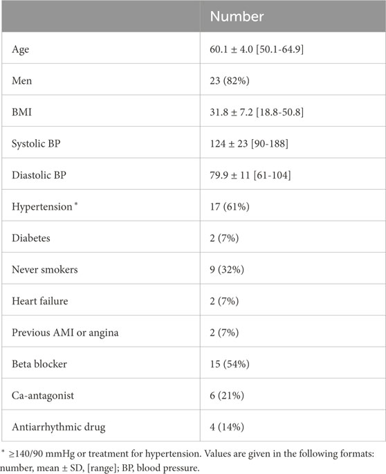
Table 1. Clinical characteristics of study population.

ECG preprocessing and QRS complex detection were performed using the CardioLund ECG parser (www.cardiolund.com). The CardioLund ECG parser classified QRS complexes based on their QRS morphology. Only QRS complexes with dominant QRS morphology were considered in the computation of the RR series.

The RR series were computed from intervals between R-peaks taken from consecutive QRS complexes with dominant QRS morphology, and the time of each RR interval was set to the time of the first R-peak in each interval. The resulting non-uniformly sampled RR series were interpolated to a uniform sampling rate of 4 Hz using piecewise cubic Hermite polynomials as implemented in MATLAB (‘pchip’, version R2023a, RRID:SCR_001622).

The AFR was used to obtain information about the atrial arrival process. Briefly, the estimation of the AFR involved the extraction of an f-wave signal by means of spatiotemporal QRST-cancellation (Stridh and Sörnmo, 2001) and estimation of an f-wave frequency trend by fitting two complex exponential functions to the extracted f-wave signal from ECG lead V1 as proposed in (Henriksson et al., 2018). The two exponential functions were characterized by a fundamental frequency f and its second harmonic, respectively; f was fitted within the range fmaxWelch±1.5 Hz, where fmaxWelch denotes the maximum of the Welch periodogram of ECG lead V1 in the range 4–12 Hz. The results for the deep breathing data have been previously presented in (Abdollahpur et al., 2022). The estimated AFR signal has a sampling rate of 50 Hz.

All steps of the extraction algorithm that are described in the following were applied to 1-min segments of the lead-specific EDR signals taken from a 1-min running window. The lead-specific EDR signals were computed with the slope range method (Kontaxis et al., 2020) for the eight ECG leads V1-V6, I, and II. Only eight out of 12 ECG leads were used, because the information in the leads III, aVF, aVL, and aVR can also be derived from lead I and II. The slope range method uses the peak-to-peak difference in the first derivative of the QRS complex to quantify the variations in the QRS morphology that are assumed to reflect the respiratory activity and are caused, for example, by periodic changes in electrode positions relative to the heart.

Only QRS complexes with dominant QRS morphology (cf. Section 2.2.1) were considered when applying the slope-range method. Further, a QRS complex was excluded as an outlier from analysis if the slope range value of any of the leads was outside the mean ± 3 std of the slope range values of that lead. The lead-specific non-uniformly sampled EDR signals were interpolated to a uniform sampling rate of 4 Hz using the modified Akima algorithm as implemented in MATLAB (‘makima’, version R2023a, RRID:SCR_001622). A matrix containing the resampled lead-specific EDR signals X′=[x1′,…,x8′]T of dimension 8 × N was constructed, where N = 240 corresponds to the length of the 1-min segment. To remove baseline-wander in X′, a Butterworth highpass filter of order 4 with a cut-off frequency of 0.08 Hz was applied separately for each lead x′. The filtered X′ was normalized to zero-mean and signals shorter than 1 min were zero-padded to create X containing 1-min segments. A set Sseg was created containing all Xi, where i = 1, … , I denotes all I possible choices of 1-min segments of the lead-specific EDR signals from one recording.

Algorithm 1.Extraction of joint-lead EDR signals.

for all Xi in Ssegdo

 Xi is whitened according to Eq. 1 to obtain Zi

 for all τj∈[10, 40] do

  obtain wj by solving the generalized eigenvalue problem of matrix pair (C̄z(τj),C̄z(0))

  compute ϵ(wj, τj, Zi) according to Eq. 2

 end for

end for

compute τ*=minτj∑Ssegϵ(wj,τj,Zi)

for all Zi in Ssegdo

 Sτ=∅

 for all τj∈[10, 40] do

  if ϵ(wj, τj, Zi) ≤ ϵ(wj, τj−1, Zi) ∨ τj= = 10 then

   if ϵ(wj, τj, Zi) ≤ ϵ(wj, τj+1, Zi) ∨ τj= = 40 then

    add τj to Sτ

   end if

  end if

 end for

 set τresp as value in Sτ closest to τ*

 obtain wresp by solving the generalized eigenvalue problem of matrix pair (C̄z(τresp),C̄z(0))

 si*=wrespTZi⋅sign∑wresp

 fresp,i= fs/τresp

end for

The joint-lead EDR signal was extracted from X using a modified version of the periodic component analysis (πCA) (Sameni et al., 2008), summarized in Algorithm 1. The matrix X was whitened for its elements to be uncorrelated and to have unit variance. The whitened lead-specific EDR signals Z were computed as

where D is the diagonal matrix of eigenvalues of the covariance matrix CX=E, and the columns of the matrix E are the unit-norm eigenvectors of CX.

The outputs of the πCA are a joint-lead EDR signal s of dimension 1 × N and its corresponding lag τ. The assumption of the πCA is that s=wTZ is a linear mixture of the whitened lead-specific EDR signals. The aim is to find a solution for s with a maximal periodic structure. The periodic structure of s is characterized by ϵ(w, τ, Z), which quantifies non-periodicity (Sameni et al., 2008) and is defined as

where s(n) is the n:th element of s. We solved the generalized eigenvalue problem (GEP) of the lag-dependent matrix pair (C̄z(τ),C̄z(0)) to obtain a full matrix V whose columns correspond to the right eigenvectors and a diagonal matrix U of generalized eigenvalues so that C̄z(τ)V=C̄z(0)VU (Sameni et al., 2008). Here, C̄z(τ)=[Cz(τ)+(Cz(τ))T+Cz(−τ)+(Cz(−τ))T]/4 for some lag τ is a modified lagged covariance matrix, which is always symmetric, unlike the time lagged covariance matrix Cz(τ)=En, where z(n) is the n:th column of Z and En indicates averaging over n. The weight vector w=[w1,…,w8]T that minimizes ϵ(w, τ, Z) is obtained as the first column of V (Sameni et al., 2008). In the present study, ϵ(w, τ, Z) is also used to quantify signal quality, where a lower value of ϵ(w, τ, Z) corresponds to a more periodic signal assumed to have a higher SNR.

As τ is unknown, ϵ(w, τ, Z) was minimized for all integer values of τ between 10 and 40, corresponding to respiration rates between 0.1 and 0.4 Hz. To improve the robustness of the πCA for signals with low quality, a τ* was determined in an intermediate step that corresponds to a global minimum of ϵ(w, τ, Z) over all 1-min segments in Sseg. It was assumed that there were no significant transient changes in respiration frequency in the clinical data and we determined two different τ* for each subject; one for normal breathing and one for deep breathing. Then, for each 1-min segment separately, a τresp was estimated as the local minimum of ϵ(w, τ, Z) closest to τ*. The respiration frequency estimate f̂resp=fs/τ̂resp results from the estimate τ̂resp and the sampling rate fs = 4 Hz and is in the range f̂resp∈[0.1,0.4] Hz corresponding to the limits set by τ. Finally, the weight vector wresp for the respiration signal extraction was obtained by solving the GEP of the matrix pair (C̄z(τresp),C̄z(0)). The extracted s=wrespTZ was normalized to unit variance. An ambiguity of πCA is that the sign of s is undetermined. The sign of the joint-lead EDR signal was selected as s*=s⋅sign∑wresp, where ∑wresp denotes the sum of the elements in the vector wresp. This was done under the assumption that all lead-specific EDR signals are in phase.

The joint-lead EDR signal extraction from Section 2.2.4 was applied to all 1-min segments X in Sseg for each patient and recording. Segments X were excluded from further analysis if they do not satisfy the following three criteria, for which a valid QRS complex has a dominant QRS morphology and is not classified as outlier based on its slope range values: i) the maximum distance between valid QRS complexes is 2 s; ii) the minimum number of valid QRS complexes in a 1-min segment is 48; iii) the minimum number of valid QRS complexes in a 1-min segment is 80% of the normal-to-normal average heart rate of the 1-min segment. After exclusion, several sets of non-overlapping 1-min segments could be created from the remaining X. Out of these, the set Sseg* that resulted in the smallest sum of ϵ(wresp, τresp, Z) was chosen, and used to produce joint-lead EDR signals XRespClin of dimension 1 × N as described in Section 2.2.4. In addition, the corresponding 1-min RR series XRRClin of dimension 1 × N was extracted from the RR series obtained in Section 2.2.1. We estimated the mean arrival rate of atrial impulses to the AV node μ̂ as 1000/AFR̄, where AFR̄ is the average AFR-trend within each of the selected 1-min windows as described in Section 2.2.2. To match the dimensions of XRRClin and XRespClin, μ̂ was then repeated N times to produce XAFRClin of dimension 1 × N. From the clinical data, a maximum of five non-overlapping 1-min long segments in normal breathing and one segment in deep breathing was obtained for XRRClin, XRespClin and XAFRClin.

The atrioventricular node is modeled by a network of 21 nodes (cf. Figure 1). The presented AV node model was initially proposed in (Wallman and Sandberg, 2018), updated with minor modifications in (Karlsson et al., 2021), and extended using constant scaling factors AR and AD for the refractory period and conduction delay to account for the effect of changes in autonomic modulation in (Plappert et al., 2022). The slow pathway (SP) and fast pathway (FP) are described by two chains of 10 nodes each, which are only connected at their last nodes. Impulses enter the AV node model simultaneously at the first node of each pathway. Within the pathways and between their last nodes, the impulses are conducted bidirectionally to allow for retrograde conduction. The last nodes of the two pathways are connected to an additional coupling node (CN), through which the impulses leave the model.

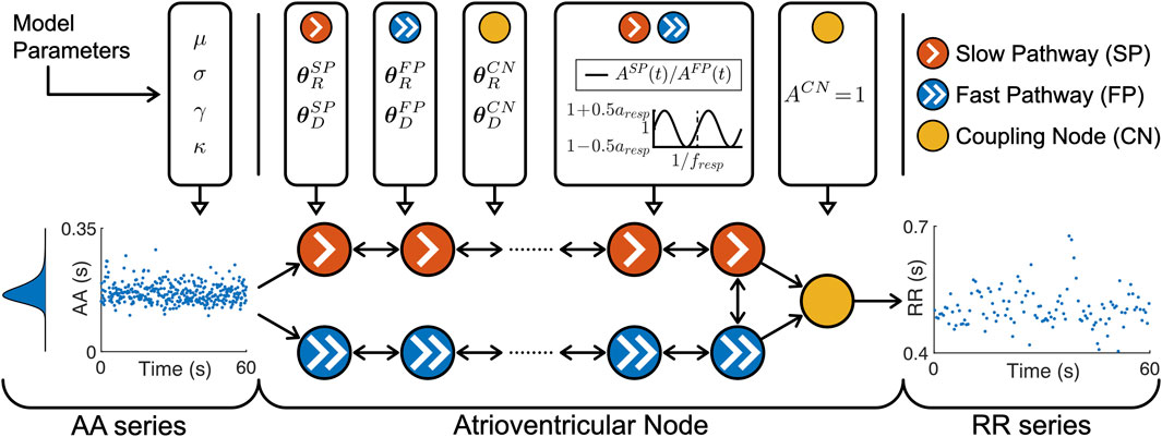
Figure 1. A schematic representation of the AV node model. Retrograde conduction was possible within the AV node model. For simplicity, only a subset of the ten nodes in each pathway is shown. Note that the atrioventricular node used different θRP and θDP for the three different pathways, the same time-varying AP(t) for SP and FP and a constant ACN = for CN.

Each node represents a section of the AV node and is characterized by an individual refractory period RP(Δtk,AP(t),θRP) and conduction delay DP(Δtk,AP(t),θDP) defined as

Where P ∈ denotes the pathway. The refractory period and conduction delay are defined by fixed model parameters for the refractory period θRP and conduction delay θDP as well as model states for the diastolic interval Δtk and respiratory modulation AP(t). Each pathway has a separate set of fixed model parameters for the refractory period θRP= [RminP, ΔRP, τRP] and conduction delay θDP=[DminP, ΔDP, τDP], where RminP is the minimum refractory period, ΔRP is the maximum prolongation of the refractory period, τRP is a time constant, DminP is the minimum conduction delay, ΔDP is the maximum prolongation of the conduction delay and τDP is a time constant. For clarity, the notation of RP (⋅, AP(t), ⋅) and DP (⋅, AP(t), ⋅) are specified with dots when the replaced parameters or model states are currently not discussed.

The scaling factor AP(t) accounts for the effect of changes in autonomic modulation on the refractory period RP⋅,AP(t),⋅ and the conduction delay DP⋅,AP(t),⋅. The time-varying scaling factor AP(t) is common between the SP and FP, defined in Eq. 5 as

with a constant respiratory frequency fresp and peak-to-peak amplitude aresp. The scaling factor of the refractory period and conduction delay of the CN is described by ACN = 1 and not modulated by respiration.

The electrical excitation propagation through the AV node is modeled as a series of impulses that can either be conducted or blocked by a node. An impulse is conducted to all adjacent nodes, if the interval Δtk between the k:th impulse arrival time tk and the end of the (k–1):th refractory period, computed as

is positive. Then, the time delay between the arrival of an impulse at a node and its transmission to all adjacent nodes is given by the conduction delay DPΔtk,⋅,⋅. If Δtk is negative, the impulse is blocked due to the ongoing refractory period RPΔtk−1,⋅,⋅. After an impulse is conducted, RPΔtk,⋅,⋅ and DPΔtk,⋅,⋅ of the current node are updated according to Eqs 3, 4, 6. Details about how the impulses are processed chronologically and node by node, using a priority queue of nodes and sorted by impulse arrival time, can be found in (Wallman and Sandberg, 2018).

The input to the AV node mode is a series of atrial impulses during AF, with inter-arrival times modeled according to a Pearson Type IV distribution (Climent et al., 2011a). The AA series is generated with a point process with independent inter-arrival times and is completely characterized by the four parameters of the Pearson Type IV distribution, namely, the mean μ, standard deviation σ, skewness γ and kurtosis κ.

The output of the AV node model is a series of ventricular impulses, where tqV denotes the time of the q:th ventricular impulse. As the refractory period RPΔtk,⋅,⋅ and conduction delay DPΔtk,⋅,⋅ are history-dependent, the first 1,000 ventricular impulses leaving the AV node model are excluded from analysis to avoid transient effects.

For the training and validation, a dataset with 2 million unique parameter sets was generated. This dataset was divided into 20 datasets with 100,000 parameter sets each, where a dataset was either used for training or validation of one of ten realizations of the convolutional neural network (CNN) that is described in Section 2.4.2. Simulations were performed with each parameter set using the AV node model described in Section 2.3.1. For each simulation, a series of 11,000 AA intervals was generated using the Pearson Type IV distribution, defined by the four parameters μ, σ, γ, and κ. The parameter μ was randomly drawn from U[100,250] ms and σ was randomly drawn from U[15,30] ms. The parameters γ and κ were kept fixed at 1 and 6, respectively, since they cannot be estimated from the f-waves of the ECG (Plappert et al., 2022). Negative AA intervals were excluded from the impulse series. The model parameters for the refractory period θRP and conduction delay θDP of the SP and FP were drawn from bounded uniform distributions and the model parameters of the CN were kept fixed according to Table 2. The given ranges were in line with our previous work (Plappert et al., 2022). The model parameters for the respiration-induced autonomic modulation and simulated respiration signal that are used in Section 2.3.3 were also drawn from bounded uniform distributions, with aresp randomly drawn from U[−0.1,0.5], fresp randomly drawn from U[0.1,0.4] Hz and η randomly drawn from U[0.2,4]. For testing, another dataset with 2 million unique parameter sets was generated using the same ranges listed above, except for aresp, which was randomly drawn from U[0,0.4].

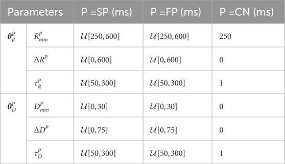
Table 2. AV Node model parameters used for simulated data.

When sampling, initially a value for aresp was drawn from a uniform distribution. To exclude non-physiological parameter sets from the dataset, we resampled the rest of the parameters until the following five selection criteria were met: 1) the slow pathway in every parameter set must have a higher conduction delay DSPΔtk,⋅,⋅>DFPΔtk,⋅,⋅ and lower refractory period RSPΔtk,⋅,⋅<RFPΔtk,⋅,⋅ than the fast pathway for all Δtk; 2) the resulting average RR interval has to fall within the range of 300 ms–1,000 ms, which corresponds to heart rates between 60 bpm and 200 bpm; 3) the resulting root mean square of successive RR interval differences (RR RMSSD) has to be above 100 ms; 4) the resulting sample entropy of the RR series has to be above 1; 5) the relative contribution of the respiration frequency in the frequency spectrum of the RR series with zero-mean FRR(fresp)/∑fFRR(f) has to be below 7% to exclude RR series with visible periodicity. Note that the frequency spectrum is computed from the RR series with 240 samples and the sampling rate of 4 Hz.

Similar to the clinical data described in Section 2.2.1, RR series were computed from intervals between the simulated ventricular impulses, and the time of each RR interval sample was set to the time of the first ventricular impulse. The resulting non-uniformly sampled RR series were interpolated to a uniform sampling rate of 4 Hz using piecewise cubic hermite interpolating polynomials as implemented in MATLAB (‘pchip’, version R