We generated the simulated data from the current RefSeq database using Mason v0.1.2 [30] with the option “illumina -pi 0 -pd 0 -pmms 2.5 -s 17 -N 2000000 -n 100 -mp -sq -hs 0 -hi 0 -i”, which simulated two million 100-bp read pairs with 1% error rate. We further filtered the reads from the sequences without taxonomy information and kept the first one million read pairs as the final simulated data set. We also obtained one million randomly selected 100-bp read pairs using the simulator ART v2.5.8 [31] with Illumina profile setting (“art_illumina -ss HS25 -m 1000 -s 100 -l 100 -f 0.003”) followed by the same filtration procedure as was used for Mason. The error rate of Art-generated simulated data was estimated to be around 0.15% by examining the aln file produced by Art. In addition to our own simulated data, we downloaded the 10 simulated samples from the CAMI2 Challenge datasets at https://frl.publisso.de/data/frl:6425521/strain/short_read/ by lexicographical order, i.e. sample_0 to sample_9. For the bacteria WGS data, we first downloaded the RunInfo from NIH NCBI SRA using the search word “(“Bacteria”[Organism] OR “Bacteria Latreille et al. 1825”[Organism]) AND (“2022/01/01”[MDAT]: “2023/08/01”[MDAT]) AND (“biomol dna”[Properties] AND “strategy wgs”[Properties] AND “platform illumina”[Properties] AND “filetype fastq”[Properties])”. Then based on whether the species or genus is present in the RefSeq database, we randomly pick 100 SRA IDs (Additional file 1: Table S3), without repeating species or genus, for species-in and species-not-in evaluations, respectively.

We benchmarked the performance of Centrifuger v1.0.1, Centrifuge v1.0.4, and Kraken2 v2.1.3, Ganon v2.0.0, and KMCP 0.9.4 in this study. For the application on long-read data sets, we also tested MetaMap with GitHub commit ID 633d2e0 and Taxor v0.1.0. Taxonomy information and microbial genomes were downloaded using the “centrifuger-download” script in June 2023. Each classifier was used to build its own index on dustmasked [49] genome sequences. Kraken2 used its own built-in masking module. Though we used Ganon v2.0.0 in evaluations, we failed to create the index with the hierarchical interleaved bloom filter data structure implemented in this version [50]. Therefore, we used the index based on the interleaved bloom filter (--filter-type ibf) for Ganon, and we referred to this method as “Ganon” rather than Ganon2. The commands used to run each method are listed in Additional file 1: Table S4. Methods like Centrifuge, Ganon, and KMCP might report multiple equally good taxonomy IDs for a read, and we merged them into LCAs before the evaluations. Ganon’s default option for coalescing the taxonomy IDs of a multiple-classified read is to reassign the read to the taxonomy ID with the highest abundance inferred by the EM algorithm using the initial classifications. This approach substantially improves Ganon’s classification sensitivity at lower taxonomy levels, leading to a higher F1 score. For example, in the Mason-generated simulated data, Ganon with reassignment’s F1 score at the species level was 1.3% and 12.1% higher than Centrifuger’s and Ganon using LCA’s, respectively (Additional file 1: Fig. S8). We implemented a similar workflow to reassign the multiple-classified reads from Centrifuger. Specifically, we ran Centrifuger with “-k 5” so that the initial classification for a read could include up to five equally good classification results. We then calculated the abundance for each taxonomy ID in the taxonomy tree based on the number of reads classified to this taxonomy node and its subtree. For a multiple-classified read, we included its count starting from its LCA. Lastly, we reassigned the taxonomy ID with the highest abundance among the initial results to a read as the final classification result. When there were multiple highest-abundance taxonomy IDs for a read, we took their LCA as the final result. We observed this reassignment strategy without the EM algorithm improved Centrifuger’s classification results at lower taxonomy levels too, with the F1 score 2.7% higher than Ganon’s reassignment results at the species level (Fig. S8). However, the strategy of hard reassignment based on the taxonomic profiling result may result in systematic underestimations of taxa with lower abundances. Therefore, we continue to utilize the LCA strategy to process multiple classified reads, where the results can be directly used for downstream analyses, including taxonomic profiling.

All the benchmarks were conducted on the 2.8 GHz AMD EPYC 7543 32-core processor machine with 512 GB memory. The memory footprint was measured as the “Maximum resident set size” value from the “/usr/bin/time -v” command. When measuring speed, each classifier was run four times. The reported classification speed was calculated by taking the fastest runtime after excluding index loading time.

Run-block compressed sequence is a compact data structure supporting rank queries for any position in a sequence. For the input sequence T of length n and alphabet set \(\Sigma\) of size \(\sigma\), we first partition T into equal-size substrings (blocks), \(_,_,\dots ,_\), where \(m=\lceil \frac\rceil\) and \(b\) is the block size. The first component of the run-block compressed sequence is a bit vector \(_\) of size m indicating whether the corresponding block is a run block, i.e., a block consisting of one alphabet character repeated b times. We will then split T into two substrings, by concatenating run blocks and non-run blocks, i.e., \(_^}=__}__}\dots __}, _=__}__}\dots __}\), and \(__}\) is the k-th run blocks in T with the alphabet \(__}\). In the notation, we will use the subscript “R” to denote run-block compressed sequence, and “P” to represent the plain uncompressed sequence. Since the last block can still be determined as a run or non-run block even if it is shorter than \(b\), we can assume that \(n\) is divisible by \(b\) for simplicity. \(_^}\) can be losslessly represented as \(_=__}__}\dots __}\), where \(\left|_\right|=\frac_^}|}\). The space saving comes from using one character to represent a run block of size b, a strategy we call run-block compression. For example, for a sequence T = “AAAAACGTAAAA”, when b = 4, it will be split into “AAAAAAAA” and “ACGT” guided by \(_=101\). For the subsequence formed by the run blocks, we will use one character to represent each block in it. Therefore, the example sequence T will be represented by two sequences \(_\)=“AA” and \(_\)=“ACGT”, reducing the original length from 12 to 6 characters (Fig. 1). We next show that run-block compression allows fast rank queries and sublinear space usage as the repetitiveness in the sequence increases. The rank query is the core operation in LF mapping during the backward search in FM-index.

Theorem 1 The time complexity for rank query on run-block compressed sequence is \(O(log\sigma )\).

Proof: We will use the function \(_(i, T)\) to denote the rank for the alphabet c at position i of text T, where the index is 1-based. Equivalently, \(_(i, T)\) counts the number of c’s that occur before T[i], including T[i]. We can decompose the \(_(i, T)\) to the sum of corresponding ranks with respect to \(_\) and \(_\). There are two cases, depending on whether i is in a run block or not. Let k denote the block containing i, namely \(k=\lceil\frac\rceil\). We compute the number of run blocks and non-run blocks before the block containing k as \(_=_\left(k,_\right), \mathrm\space\overline_}=_\left(k,_\right)=k-_\), respectively. The \(_\left(k,_\right)\) is the conventional rank query on bit vectors counting the number of 1 s before or on position k in BR. With these notations, we can write the equations to compute \(_(i, T)\).

When i is in a run block, i.e., \(_[k]=1\), we have:

$$_\left(i, T\right)=b\left(_\left(_,_\right)\right)+_\left(\overline_}b, _\right)+__\left[_\right]=c}\left(\left(i-1\right)\%b+1-b\right)$$

Where \(__\left[_\right]=c}\) is an indicator that equals 1 if the subscript is true and equals to 0 otherwise. The last term is the special treatment if i is in a run block with alphabet character c. When i is in a non-run block, we have:

$$_\left(i, T\right)=b\left(_\left(_,_\right)\right)+_\left(\left(\overline_}-1\right)b+(i-1)\%b+1, _\right)$$

If we apply the wavelet tree to represent \(_\) and \(_\), then \(_(i, T)\) can be answered by at most two wavelet tree rank queries, one rank query on bit vector \(_\), and one wavelet tree access on \(_\). Therefore, the total time complexity is \(3O(log\sigma )+O\left(1\right)=O(log\sigma )\).

The naïve implementation for calculating \(__\left[_\right]=c}\) is to access the value of \(_\left[_\right]\), requiring \(O(log\sigma )\) time if using wavelet tree. We note that the \(__\left[_\right]=c}\) can also be inferred during the wavelet tree’s rank query on \(_\), by checking whether the bits labeling the relevant root-to-leaf path form the bit representation for c. This strategy further accelerates the \(_(i, T)\) operation, and is also applicable to other compressed sequence representations, including RLBWT.

Theorem 2 The space complexity of run-block compressed sequence is \(O(\frac}}\sigma )\) bits, where \(l=\frac\) is the average run length and r is the number of runs in the sequence.

Proof: The key observation is that each non-run block contains at least one run head. Therefore, we have at most r non-run blocks. As a result, the minimum length of \(_\) is \(\frac-r\), and the maximum length of \(_\) is \(rb\). The length of the \(_\) is \(\frac\).

We can use wavelet trees to represent the run-block subsequence and the plain subsequence. Let \(A\) be the number of bits to represent one character in the wavelet tree, then the asymptotic total space usage in bits is \(\frac+A\left(\frac-r\right)+Arb\), where the terms are for \(_\), \(_\), and \(_\), respectively. We can rewrite the space usage bound as:

which is minimized when \(b=\sqrt}\). Because b is an integer, we take the block size as \(^=\lceil\sqrt}\rceil\). Substituting this for \(b\), we have:

$$S\left(^\right)=Ar\lceil\sqrt}\rceil+\frac}\rceil}-Ar<\sqrt+\sqrt=O\left(A\sqrt\right),$$

where the inequality is based on\(\sqrt}\le \lceil\sqrt}\rceil<\sqrt}+1\). We can rewrite \(S\left(^\right)\) by using the definition of \(r=\frac\), obtaining \(S(^)=O\left(A\frac} \right).\) To ensure the worst rank query time on the data structure is small, the wavelet tree is in the shape of a balanced binary tree in our implementation, and \(A=O(}\sigma )\). Further space could be reduced if we use techniques like Huffman-shaped wavelet tree [51], and A will be \(O\left(_\left(_\right)\right)\) and \(O\left(_\left(_\right)\right)\) for TR and TP, respectively, where H0 is the Shannon entropy of the sequence.

The \(^\) found in the proof is to bound the worst-case space usage, where each non-run block has exactly one run head in the middle. The optimal block size can be different. For example, when every run has an identical length, the optimal block size is \(\frac\) and every block is run-block compressible, yielding \(O\left(\frac}\sigma \right)\)-bit space complexity. To find the appropriate block size efficiently, we search the size of powers of 2, e.g., 4, 8, 16,.., and select the block size \(\widehat\) with the least space usage among them. Suppose \(}^\) is the smallest power of 2 that is larger or equal to the block size \(^\) defined in the proof, then we have \(^\le \widehat}^\le 2^\). Therefore, \(S\left(\widehat\right)\le S\left(}^\right)\le 2Ar^+\frac^}-Ar\le 2S\left(^\right)+Ar=O\left(\frac}\right)\), where the second inequality is by applying \(^\le \widehat^\le 2^\). Therefore, the block size inferred from inspecting powers of 2 is not a bad estimator and gives the same asymptotic space usage as \(^\) in the worst case. Furthermore, since \(Ar\le A\sqrt<S(^)\), \(S\left(\widehat\right)\) is no more than three times of the \(S(^)\). To reduce the bias of the sparse search space, we also inspect the space usage of block sizes \(^\) and \(\frac}\) before making a final decision. When \(l\) is small, the block size minimizing the overall space usage is the length of the genome (TP = T), and run-block compression is equivalent to the wavelet tree representation. In practice, Centrifuger uses the first one million characters of the BWT sequence instead of the full sequence to infer the block size.

Centrifuger uses the blockwise suffix sorting algorithm [52] to build its index, as in Bowtie [53] and Centrifuge. The advantage of blockwise suffix sorting is to control the overall memory footprint and parallelize the construction procedure. The array that holds the BWT sequence is pre-allocated, and the sequence is filled in block-by-block as blocks of the suffix array are constructed. Another important component in the FM-index is the sampled suffix information. During construction, the index stores the genome coordinate information for every 16th offset on the BWT, which can be adjusted by the user. After that, the offsets are transformed into sequence IDs and using a bit-efficient representation of the IDs. For example, the RefSeq prokaryotic genome database contained 75,865 sequences (including plasmids) from 34,190 strains with complete genomes, so sequence IDs can be distinguished by a 17-bit integer. Instead of saving the IDs in an array of 32-bit integers, the bit patterns are stored consecutively without any wasted space. Therefore, the total size for the bit-compact array for the sampled ID list is 17·m bits, or 0.26·m 64-bit words, where m is the number of sampled IDs.

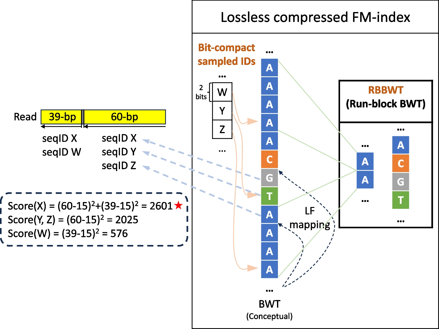
For taxonomic classification, Centrifuger follows Centrifuge’s paradigm by greedily searching for semi-maximal exact matches, where only one side of a match cannot be extended to form a longer match to the database (Fig. 1). For each read pair, Centrifuger searches the matches twice, one using the forward strand and the other using the reverse-complement strand. Using the forward strand search as an example, Centrifuger starts from the last position of the read and extends the match backward as much as possible using LF mapping until the match cannot hit any sequence in the index. In the example in Fig. 1, the first match is the right-most 60 bp. Centrifuger will then skip the next base on the read, as a putative variant or sequencing error, and start a new search. As a result, the next search starts from the 62nd bp, counting from the right end, and finds a match of length 39.

To find the best taxonomy ID for the read, Centrifuger scores the sequence IDs retrieved from the matches. Let \(_\) denote the length of a match \(M\). Centrifuger will filter a short match \(M\) if \(2n/^_}>0.01\), as it is likely a random match. For example, we kept the matches with lengths greater or equal to 23 as valid matches when classifying reads using the 140 GBp RefSeq prokaryotic database. Each valid match \(M\) of length \(_\) will contribute a score \(_-15\right)}^\) to the corresponding strand, and the matches from the less-scored strand will be removed. Centrifuger resolves sequence IDs contained in each valid match by using LF-mapping in the compressed FM-index to find sampled sequence IDs. Specifically, each match \(M\) corresponds to an interval on the BWT sequence, denoted as \(\left[_,_\right]\), then we will resolve the sequence ID for each position on the BWT sequence between \(\left[_,_\right]\), by applying LF-mapping. The LF-mapping procedure for resolving the position \(p\in \left[_,_\right]\), terminates when it reaches a position \(p^\) on the BWT sequence with a sampled sequence ID, i.e., \(p^\space mod\space 16=0\) with the default parameter. The sampled sequence ID at \(p^\) is the sequence ID corresponding to \(p\). In the example of Fig. 1, the Centrifuger found the first 60-bp exact match \(_\) hit sequences with IDs X, Y, and Z, and the second 39-bp exact match \(_\) were from sequence IDs W and X. If both strands have an equal score, the sequence ID will be resolved for both strands. For each resolved sequence ID, Centrifuger will sum up its scores across the matches using the formula \(}\left(}\space I\right)=_}\space I}_-15\right)}^\), where \(M\in \space} I\) means the match \(M\) is found in the sequence with ID \(I\). In the example of Fig. 1, the score for sequence ID X is \(^+^=2601\) as both matches hit this sequence. This scoring function was empirical and was designed during the development of Centrifuge. The sequence IDs with the highest score and their corresponding taxonomy IDs will be reported as the final classification result for the read, where the example read in Fig. 1 is classified to the sequence X. When the number of highest-scoring sequence IDs is more than the report threshold that can be specified by the user (default 1), Centrifuger will merge the IDs to their LCAs in the taxonomy tree until the number is within the threshold.

For a match that hits many sequences in the database, i.e., \(_-_+1\) is large, Centrifuger will resolve the sequence IDs for at most 40·report_threshold entries evenly distributed in the BWT interval. For example, if \(_=100\) and \(_=490\), then Centirufger will resolve the 40 sequence IDs for positions at 100, 110, 120,.., 480, and 490 on the BWT sequence with the default setting. Though this is a heuristic that can cause the algorithm to miss the true genome of origin, it is likely to generate scores for sequences in the same phylogeny branch and may help identify the correct taxonomy IDs at higher levels. This is the main difference between Centrifuge and Centrifuger in the classification stage, where Centrifuge ignores a match \(M\) if \(_-_+1 >200\) with the default setting.

In addition to the run-block compression, we designed another compression scheme called hybrid run-length compression, using run-length compression for each fixed-size block. Hybrid run-length compressed BWT uses the same amount of space as the wavelet tree representation when the repetitiveness of the sequence is low, and its space usage converges to the RLBWTs when the repetitiveness grows. In our implementation, a block is marked as run-length compressible (BR = 1) if its average run-length is more than six based on the comparison between RLBWT and wavelet tree (Fig. 2A, B). The substrings from blocks are separated into two subsequences based on BR, and the subsequences will be concatenated into two sequences, TR and TP, respectively. TR will be compressed by the run-length method as in RLBWT, and TP will be represented as a wavelet tree. The block size is inferred in the same fashion as in RBBWT. The rank query on the hybrid run-length compressed sequence is like the run-block compression, where we combine the ranks from TR and TP, making it slower than the rank query on RLBWT. The idea of hybrid run-length compression is similar to the wavelet tree when using fixed-block boosting [54]. Our implementation avoids explicitly recording the accumulated count at the beginning of a block and is therefore well suited to mildly repetitive sequences needing small blocks. For example, the block size of the hybrid run-length compressed BWT was only 12 for the genus Legionella’s genomes. Despite being less computationally efficient than other representations, the hybrid run-length compressed BWT is flexible and allows methods to handle various texts with a wide range of repetitiveness without altering the underlying data structure.