In this work, we address the problem of extracting a set of template instances from unstructured text. We tackle this problem from two different perspectives and present two approaches solving the same problem: 1) an extractive approach and 2) a generative approach. An illustration of both approaches can be found in Fig. 1.

Fig. 1

Illustration of both described approaches starting with the tokenized input and ending with the generated template instances

The used data model captures the design and key results of an RCT by way of 10 different templates consisting of a total of 85 different slots that capture various aspects of the PICO elements in a structured way. These templates are based on the C-TrO Ontology that has been designed to support use cases related to the aggregation of evidence from multiple clinical trials [15]. The mean number of slot fillers per template is shown in Table 1. A template \(t_i\) is defined by a type \(i \in \mathcal L\) and a set of slots \(\mathcal S_i = \bigcup _j s_\), where \(s_\) denotes slot j of template \(t_i\), \(\bigcup _j\) this way denotes the set union over all slots j and \(\mathcal L\) denotes the set of all template types. A template is instantiated by assigning slot-fillers to its slots, where a slot-filler can be either a text span from the input document or a template instance, depending on the slot. Figure 2 visualizes the used data model. In the following subsections, we describe the extractive and the generative approach in more detail.

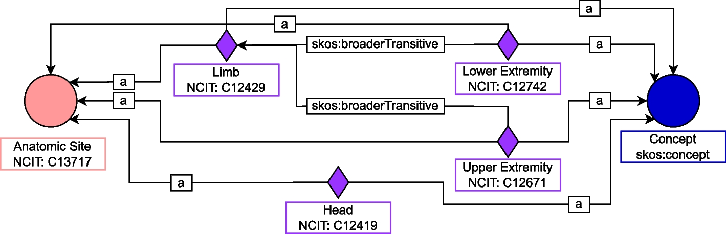
Table 1 Mean and standard deviation of the number of slot fillers per template in the used dataset, separated by type of disease. Numbers rounded to two decimal placesFig. 2

Schema of the PICO data model used in the experiments

Extractive approach

Our extractive approach is based on the Intra-Template Compatibility (ITC) approach [14], which adopts a two-step architecture: In a first step, all textual slot-fillers are extracted from the input document, followed by a second step, which assigns the extracted slot-fillers to template instances. The extraction of slot-fillers and their clustering and assignment are described in the “Extraction of textual slot-fillers” and “Assignment of textual slot-fillers to template instances” Sections, respectively.

Encoding of the input document

The ITC approach uses BERT (Bidirectional Encoder Representations from Transformers) [53] to compute a contextualized representation of each token \(w_i\) of the input document \(d=(w_1,\ldots ,w_n)\). As the length of RCT abstracts typically exceeds the maximum number of tokens of most BERT implementations, the authors of ITC split the document into consecutive chunks and process each chunk separately. However, this approach treats each chunk as an isolated unit and hence the model is not able to learn token representations which incorporate the context of the full input document. Therefore, we adopt the Longformer [16] approach as well as the Flan-T5 model [17] to learn full-document contextualized representations \(\textbf_i \in \mathbb R^d\) (with \(d = 768\) for both T5 and Longformer models) for each token \(w_i\) of the input document, where d is the output dimension of the encoder of the respective model.

Extraction of textual slot-fillers

The ITC approach extracts slot-fillers from the input document by predicting start and end tokens of slot-fillers, followed by a step which joins the predicted start and end tokens. This is realized by training two linear layers which take the contextualized representation \(\textbf_i\) of the tokens \(w_i\) as input and predicts whether or not this is a slot-filler start or end token, respectively:

$$\begin \textbf_ = \text (\textbf_s \textbf_i + \textbf_s) \qquad \textbf_s \in \mathbb R^, \quad \textbf_s \in \mathbb R^ \end$$

(1)

$$\begin \textbf_ = \text (\textbf_e \textbf_i + \textbf_e) \qquad \textbf_e \in \mathbb R^, \quad \textbf_e \in \mathbb R^ \end$$

(2)

where \(\mathcal S = \bigcup _i \mathcal S_i \cup \\) is the set of all slots including the special no-slot label \(\mathbb O\) which indicates that a token is not classified as a start/end token of a slot-filler. The vectors \(\textbf_\), \(\textbf_\) denote the predicted probability distribution over the slots that a token \(w_i\) is the start/end of the respective slots. The final prediction is determined by the \(\arg \max\) operation.

The predicted start/end tokens are joined sentence-wise by minimizing the distance between start and end tokens in terms of tokens in between. More precisely, for a given sentence, we first collect all predicted start and end tokens. For each predicted start token \(w_s\), at position i we seek an end token \(w_e\) at position \(j \ge i\) with matching label and minimal distance to \(w_s\) and assign it to \(w_s\) as its end token. Finally, we discard predicted start/end tokens which have no matching end/start token. This slightly differs from the IOB format [58], as only start and end token of a sequence are tagged and all tokens in between are classified just like tokens which are not part of any sequence. A comparison of both tagging schemes can be found in Table 2.

Table 2 Comparison of used tagging schema with the IOB format, where O represents tokens outside of a sequence and I-Frequency represents tokens which are part of a slot filler sequence of type frequency. In contrast, None represents tokens which are neither start nor end token of a slot filler, start:Frequency marks the start and end:Frequency the end of a frequency slot filler sequence

For each extracted slot-filler i with start/end tokens \(w_s\) resp. \(w_e\) with corresponding token representations \(\textbf_s\), resp. \(\textbf_e\), ITC computes a representation \(\textbf_i\) by summing the representations of the start and end tokens followed by a dense layer with ReLU [59] activation function:

$$\begin \textbf_i = \text (\textbf_r(\textbf_s + \textbf_e) + \textbf_r) \qquad \textbf_r \in \mathbb R^, \quad \textbf_r \in \mathbb R^d \end$$

(3)

The learned representations \(\textbf_i\) of the extracted slot-fillers (SFs) are then used as input to subsequent modules. In the remainder of this paper, we denote the set of all extracted slot fillers as \(\mathcal E\), where each slot filler in \(\mathcal E\) is represented by its vector representation computed by Eq. (3).

Assignment of textual slot-fillers to template instances

Typically, for some slot types like the textual slot fillers of the Outcome template, there are several slot fillers of the same type extracted from an original document. Therefore, we need a way to group these slot fillers such that actual template instances, e.g. multiple Outcome instances, can be created from these slot fillers. Deciding which slot fillers belong together is however not a trivial task.

The assignment of extracted SFs to template instances is therefore done in ITC by a clustering approach per template based on a pairwise similarity or compatibility function \(q: \mathbb R^d \times \mathbb R^d \rightarrow [0, 1]\). q scores the similarity between two SFs in the sense that they belong to the same template instance, where \(g(\textbf_i, \textbf_j)=1\) indicates maximum similarity such that \(\textbf_i\) and \(\textbf_j\) should be assigned to the same template instance. Note that \(\textbf_i\) and \(\textbf_j\) are entity representations calculated based on the contextualized embeddings generated by the used models. Thus, we can use results from the established field of (density-based) clustering to figure out the SF grouping. The similarity function q is implemented in a slightly more complex way compared to the original paper, using two linear layers with a ReLU activation function in between and followed by a sigmoid activation function:

$$\begin q'(\textbf_i, \textbf_j) & = \text (\textbf_h(\textbf_i + \textbf_j) + \textbf_h)\quad \quad \textbf_h \in \mathbb R^, \quad \quad \textbf_h \in \mathbb R^d \end$$

(4)

$$\begin q(\textbf_i, \textbf_j) & = \sigma (\textbf_s^T(q'(\textbf_i, \textbf_j)) + \textbf_s)\quad \quad \ \ \textbf_s \in \mathbb R^d, \quad \qquad \ \ \textbf_s \in \mathbb R \end$$

(5)

Note that due to the symmetry of \(+\), also q is a symmetric function, i.e. \(q(\textbf_i, \textbf_j) = q(\textbf_j, \textbf_i)\) for all pairs of \(\textbf_i, \textbf_j\). Then the mean pairwise similarity between SFs of a cluster \(C_i \subseteq \mathcal E\) is given by

$$\begin g(C_i) = \frac \sum \limits __i, \textbf_j) \in C_i \times C_i} q(\textbf_i, \textbf_j) \end$$

(6)

The score of a clustering \(\mathbb C_i = \ \}\) of SFs \(\mathcal E_i \subseteq \mathcal E\) for template \(t_i\) is the mean score of its cluster scores:

$$\begin h(\mathbb C_i) = \frac \sum \limits _ g(C_k) \end$$

(7)

The ITC approach seeks a clustering \(\mathbb C_i^*\) of \(m_i\) clusters which maximizes the score given by Eq. (7):

$$\begin \mathbb C_i^* (m_i) = \arg \max _} h(\mathbb C_i) \end$$

(8)

where \(\mathcal U_\) denotes the set of all clusterings of the set \(\mathcal E_i\) with \(m_i\) clusters. Note that the optimization objective defined by Eq. (8) is parameterized by the number of clusters \(m_i\). In order to alleviate the assumption that the number of instances of templates needs to be known a priori, we propose a clustering step to induce the number of template instances per template type using Hierarchical Agglomerative Clustering (HAC) with a threshold based on the average of values computed for the training data, namely:

After the clustering \(\mathbb C_i^*(m_i)\) has been estimated, the template instances \(t_\) are derived from those clusters \(C_j^* \in \mathbb C_i^*(m_i)\). The slot to which a SF \(\textbf_k \in C_j^*\) is assigned is given by the label assigned by the SF extraction module by Eqs. (1) and (2). In summary, the assignment of SFs to template instances is done as follows:

1.

For each template \(t_i\), the set \(\mathcal E_i \subseteq \mathcal E\) of SFs which can be assigned to instances of template type \(t_i\) is estimated.

2.

Equation (8) or Agglomerative Hierarchical Clustering is used to find some clustering of the SFs in \(\mathcal E_i\).

3.

The template instances are derived from the clusters in the clustering.

As an example, we consider the following four extracted slot fillers:

1.

PercentageAffected: 16

2.

PercentageAffected: 8

3.

TimePoint: week 24

4.

TimePoint: week 12

Additionally, we assume our trained similarity function gives us the similarities presented in Table 3.

Table 3 Example similarities/compatibilities between four slot fillers, slot types in first row have been omitted

Given these similarities and a clustering threshold of, e.g., 0.5, this results in two clusters which can be then directly used to create the corresponding Outcome template instances. These two clusters are:

1.

PercentageAffected: 16 and TimePoint: week 24

2.

PercentageAffected: 8 and TimePoint: week 12

The clustering thus provides a robust and flexible way to both determine the number of template instances to generate as well as the groups of slot fillers those instances comprise.

Generative approach

In this section we propose a simple generative approach for extracting template instances from unstructured text based on the Transformer [60] encoder-decoder model. As encoder-decoder models require the output to be a linear token sequence, the set of TIs needs to be converted into a sequence of tokens. In Section “Linearization of sets of template instances”, we present a simple recursive method for linearizing sets of TIs along a context free grammar (CFG) for describing the linearized structures. In Section “Decoding” we adopt the presented CFG for generating valid token sequences representing sets of TIs.

Transformer-based encoder-decoder models

Transformer-based [60] encoder-decoder models are seq2seq models which haven been used on a variety of natural language processing tasks like machine translation [61] and text summarization [62]. The encoder part of the Transformer learns a contextualized representation of the input tokens \(w_1, \ldots , w_n\) via multi-headed self-attention [60], converting the input sequence into a sequence of vectors \(\textbf_1, \ldots , \textbf_n \in \mathbb R^d\), where d is the dimension of the Transformer model. Then the decoder part takes the vector sequence from the encoder as input and produces an output vector sequence \(\textbf= (\textbf_1, \ldots , \textbf_n \in \mathbb R^d)\) via multi-headed cross-attention. The computational complexity of self-attention grows quadratically with the number of tokens. Beltagy et al. [16] proposed the Longformer encoder-decoder, which combines local and global multi-headed self-attention in the encoder, reducing computational complexity from \(\mathcal O(n^2)\) to \(\mathcal O(n)\).

The output vector sequence \(\textbf\) is used to compute a probability distribution over the vocabulary of the underlying model via the following equation:

$$\begin p(y_i | x, y_1, \ldots , y_ ) = \text (\textbf_i^T \textbf_ + b_i) \end$$

(9)

where \(\textbf_i \in \mathbb R^d\) is the embedding of token \(y_i\), \(b_i\) is a bias for token \(y_i\), \(\textbf_\) is the output vector of the decoder at position \((t-1)\) and d is the model dimension. The probability of token \(y_t\) at position t is conditioned on the input token sequence x and the past decoded tokens \(y_1, \ldots , y_\). This dependence is encoded through the vector \(\textbf_\) via multi-headed self- and cross-attention.

Token prediction in the decoder is done by maximum a posteriori probability (MAP) inference. Hence the predicted token at position i is given by the token with maximal posterior probability:

$$\begin y_t = \arg \max _i p(y_i | x, y_1, \ldots , y_ ) \end$$

(10)

The generative model is trained via teacher forcing by minimizing the cross entropy loss between the predicted token distribution described by Eq. (9) and the ground truth label.

Linearization of sets of template instances

As encoder-decoder models expect the output space to be token sequences, we present a simple recursive linearization procedure of template instances (TIs). First, note that TIs are described by the content of their slots (i.e., their slot-fillers), and that slot-fillers can be either text spans from the input document or other TIs. Hence the recursion base is given by the linearization of textual slot-fillers. Let \(f = w_, \ldots , w_\) be a token sequence which represents a textual slot-filler f for a slot of name SLOT. Then the linearization of this slot-filler is the token sequence itself enclosed by the special tokens [start:SLOT] and [end:SLOT], i.e. [start:SLOT] \(\odot ~w_ \odot \ldots \odot w_ \odot\) [end:SLOT], where \(\odot\) denotes the concatenation of tokens. If the slot-filler is a TI, then it is recursively linearized and the resulting token sequence is enclosed by the special tokens [start:SLOT] and [end:SLOT]. The linearization of TIs is described below.

In general, more than one slot-filler can be assigned to a slot of a TI. Therefore, we denote the complete content of a slot as a set \(\mathcal F\) of slot-fillers. As sets, in contrast to sequences, are unordered constructs by definition, the linearization of sets of slot-fillers is inherently ambiguous. To get an unambiguous order, we introduce a slot ordering operator \(\omega\) which converts sets of slot-fillers into sequences of slot-fillers according to predefined criteria (e.g. position within input document in case of textual slot-fillers). Then sets \(\mathcal F\) of slot-fillers are linearized as follows: First, we sort the elements of \(\mathcal F\) according to the sorting operator \(\omega\) and obtain a sequence F of slot-fillers. Then we linearize each slot-filler in F as described above and concatenate the resulting token sequences, respecting the ordering of slot-fillers in F.

Next, we describe the linearization of TIs. As TIs are represented by the content of their slots, the linearization of a TI has to include the linearization of its slots. However, a template does not impose any ordering of its slots, and hence the linearization order of the slots of a TI is undefined. Therefore, we introduce another ordering operator \(\Omega\) which orders the slots of a template. Then the linearization of a TI is the concatenation of the linearizations of its slots according to the ordering of its slots given by the ordering operator \(\Omega\).

Any set of TIs induces a graph with TIs as nodes and links between TIs as edges. Recall that there is a link from TI \(t_\) to TI \(t_\) iff \(t_\) is a slot-filler of \(t_\). In order to guarantee that the linearization algorithm described above is well defined, we require the induced graph to be 1) acyclic and 2) connected. The first requirement ensures that the linearization algorithm terminates, while the second ensures the absence of isolated TI, which can not be linearized.

However, choosing \(\omega\) and \(\Omega\) is only necessary for training but not for inference purposes, as the decoding allows to fill template slots in any order. Therefore, we choose arbitrary but fixed \(\omega\) and \(\Omega\) for the experiments described in the “Experimental results” Section.

A full example for a whole linearized publication template instance can be found in Listing 2 in Appendix 6. A shorter example for an intervention template instance with both textual and template slot fillers can be found in Fig. 3.

Fig. 3

Illustration of linearization of an intervention template instance

A context-free grammar for describing linearization of sets of template instances

In the following, we describe the linearization of sets of TIs (described in Section “Linearization of sets of template instances”) by a context-free grammar (CFG) which is used in the decoding process (“Decoding” Section) to constrain the generation of tokens. A CFG is defined by a 4-tuple \(\mathcal G = (N, T, R, S)\), where N is a set of non-terminal symbols, T is a set of terminal symbols, R is a set of production rules and \(S \in T\) is the start symbol of the grammar. The set of terminal symbols is defined by the vocabulary of the underlying encoder-decoder model together with some special tokens for defining the production rules R. The recursion base of the linearizations of sets of TIs is given by the linerization of textual slots which we describe by the following equation:

$$\begin \texttt := \texttt \end$$

(11)

where TEMPLATE and SLOT are placeholders for names of template and slots, respectively, TEXT is a placeholder for any token sequence from the input document and [start:SLOT], [end:SLOT] are special tokens enclosing the textual slot-filler. Eq. (11) schematically defines production rules for textual slot-fillers, and TEMPLATE is the non-terminal symbol which is used to identify the respective production rules. Note that the non-terminal symbol TEMPLATE on the right-hand side of Eq. (11) allows recursion and hence the application of more the one production rule associated with the non-terminal symbol TEMPLATE. The recursion base of production rules is given by

$$\begin \texttt := \texttt \end$$

(12)

where TEMPLATE is again a placeholder for the template name and [end:TEMPLATE] is a special token indicating the end of the linearization of the template TEMPLATE. Production rules for TIs are described by

$$\begin \texttt := \texttt \end$$

(13)

Analogously to the production rules defined by Eq. (11) for textual slot-fillers, the production rules for slots containing TIs as slot-fillers is defined by

$$\begin \texttt := \texttt \end$$

(14)

where TEMPLATE_HEAD is a placeholder for any non-terminal symbol whose associated production rules are derived from Eq. (13). Listing 1 shows the production rules for the data model used in our experiments.

Decoding

In Section “A context-free grammar for describing linearization of sets of template instances”, we presented a CFG which describes valid token sequences representing a set of TIs. In this section, we describe a simple method to constrain token prediction such that only such token sequences are generated which are valid according the CFG. For example, consider a slot Drug which can have textual slot-fillers for describing drug names for a medication. After the special token [start:Drug] has been predicted, we know that the set of next possible tokens would consist of all tokens from the input document plus the special token [end:Drug]. This information is encoded by the CFG, and the decoding method described in this section uses this information to constrain token prediction.

In this paper, we slightly generalize the constrained decoding approach of Lu et al. [20] to arbitrary right-linear CFGs by applying a strategy similar to recursive descent parsing.

Beginning with a start symbol, in our case PUBLICATION_HEAD, the set of possible next tokens is calculated in each decoding step. This set is then used to generate a mask for the model vocabulary to discard all tokens which would not comply with the production rules of the CFG. From the remaining tokens, we select the token with the maximum value in a greedy fashion. The implementation of a beam search to optimize the decoding output even more remains for future work.

To keep track of the decisions and possible next tokens, a stack data structure is used to guide the decoding. Whenever a start token of a slot like [start:NumberAffected] is chosen as the decoded token, this decision is saved by adding this to the decoding stack. This is then used to constrain the tokens in the next step to be only those which can follow a [start:NumberAffected] token. Similarly, when an end token like [end:NumberAffected] is chosen, the top stack element is removed from the stack.

This way, the decoding is guided to comply with the requirements imposed by the CFG and this way ensuring the output can then be parsed into actual TIs.