1 Introduction

Structural and functional magnetic resonance imaging have held promise as a potential biomarker for diagnosing patients with neurological and neuropsychiatric conditions. Functional magnetic resonance imaging (fMRI), a technique that detects changes in blood flow associated with increased neural activity, has been found informative in identifying functional impairments in brain disorders. Resting-state fMRI (rs-fMRI), which examines the spontaneous fluctuations of blood-oxygen levels in the absence of neuronal stimulation, has been increasingly utilized as a biomarker for various brain disorders. This technique explores the intrinsic functional characteristics of the brain network, revealing alterations in functional connectivity (FC) (can be expressed in terms of the statistical relationship between two time series from different brain regions) in patients with brain disorders compared to healthy individuals. For instance, research on autism spectrum disorder revealed a reduction in FC between the posterior superior temporal sulcus and amygdala, linked to voice perception and language development, as discovered by Alaerts et al. (2015). Additionally, Gotts et al. (2012) showed decreases in limbic-related brain regions associated with social behavior, language and communication. FC abnormalities also have been reported in patients with Alzheimer's disease (AD) when compared to healthy controls, particularly within the default mode network (DMN), a network that is involved in memory tasks among other functions. These disruptions occur between the precuneus and posterior cingulate cortex with the anterior cingulate cortex and the medial prefrontal cortex, as indicated by Brier et al. (2012) and Griffanti et al. (2015). Machine learning (ML) or deep learning algorithms have been extensively used to improve diagnostic results, leveraging the FC abnormalities in patients as informative features. These algorithms have been proven to significantly contribute to more accurate and early detection of brain disorders (Deshpande et al., 2015; Rabeh et al., 2016; Zou et al., 2017; Qureshi et al., 2019; Lanka et al., 2020; Ma et al., 2021; Yan et al., 2021), providing a rapid and automated tool for future diagnostic applications.

Beside fMRI, structural or anatomical MRI can also be useful in ML applications by offering morphometric information about the brain, such as volumes of white matter (WM) and gray matter (GM), cortical thickness, etc. Measuring hippocampal volume, a metric derived from structural MRI, has been shown to discriminate not only between AD patients and healthy subjects, but also among individuals with other dementia-related disorders (Schuff et al., 2009; Vijayakumar and Vijayakumar, 2013). Diffusion tensor imaging (DTI) is one of the modality that can reveal structural information about brain connectivity by measuring the direction and magnitude of water diffusion. DTI has the capability to define structural connectivity (SC) based on the fibers that link each pair of brain regions. Research has demonstrated that analyzing connectivity patterns through DTI-based SC can effectively distinguish individuals with brain disorders. This approach offers valuable insights into the irregularities with neural pathways, contributing to the identification and understanding of various neurological conditions (Tae et al., 2018; Billeci et al., 2020). Many studies have illustrated that enhancing diagnostic accuracy is achievable by incorporating multimodal information from both functional and structural connectivity data (Libero et al., 2015; Pan and Wang, 2022; Cao et al., 2023). However, the practical application of ML is still impeded by challenges such as high-dimensional spaces and imbalanced datasets in real-world scenarios. In addressing these obstacles, the implementation of generative adversarial network has shown promise, offering a potential solution to mitigate these issues and enhance the effectiveness of ML approaches.

Generative adversarial network (GAN) was proposed by Goodfellow et al. (2014). The concept is inspired by the zero-sum game in game theory (where one agent's gain is another agent's loss). GAN is a generative model that learns to produce synthetic images from random noise z derived from the prior distribution p(z), which is commonly Gaussian or uniform distribution. With the impressive performance shown in image generation, its unique and inspiring adversarial characteristic to discover data distributions is also exploited in clinical applications wherein GAN is being used for classification, detection, segmentation, registration, de-noising, reconstruction and synthesis. Here, we provide a brief overview of the vanilla GAN (the original GAN) and its extensions that have been developed and commonly used in clinical applications to brain disorders.

Data scarcity and imbalanced data (the number of healthy individuals often exceeds the number of unhealthy ones) are common challenging issues in classification task. Traditional data augmentation methods such as flipping, rotation, cropping, scaling and translation generate data sharing a similar distribution with the original ones, leading to the performance of the model does not improve. Since the topology of brain networks plays a pivotal role in characterizing information flow and communication between different brain regions, these methods, while effective for regular image data, can inadvertently distort the connectivity patterns encoded in FC brain network data. While certain data augmentation techniques, such as Synthetic Minority Over-Sampling (SMOTE) (Eslami and Saeed, 2019; Eslami et al., 2019) or Adaptive synthetic sampling (ADASYN) (Koh et al., 2020; Wang et al., 2020) has been proposed tackle the challenge of data imbalance, they often rely on linear interpolation for data sampling. This may introduce artifacts as well as data redundancies. Consequently, these methods might not be optimally effective for robust data augmentation. GAN can be used as an alternative data augmentation technique and it have been proved to improve the performance of the model. Zhou et al. (2021) proposed a GAN model that can generates 3 T imaging data from 1.5 T data collected from Alzheimer's Disease Neuroimaging Initiative (ADNI) dataset and they used both the real 3 T and synthetic 3 T data to classify healthy subjects with Alzheimer's patients. However, to apply 2D convolution of CNN in more appropriate way, Kang et al. (2021) divided the 3D images into various 2D slices and applied ensemble method to produce the best results.

However, those methods are still applied on 3D imaging data, which cost a large amount of computational resources. To solve this problem, a GAN framework (Yan et al., 2021) was proposed with the generator that can take a random noise input and produce synthesis functional connectivity (FC). The model used the BrainNetCNN (Kawahara et al., 2017) as discriminator to extract meaningful features and it can perform two tasks simultaneously: testing the authenticity of the output data and classifying which label the data belong to. Other approaches also generated FC constructed from independent component analysis (Zhao et al., 2020) or combined variational autoencoder (VAE) with GAN (Geng et al., 2020) to give more control to the latent vectors.

There are also a number of obstacles occurring when we train a GAN model. Mode collapse is one of the most difficult problem in training GAN model. This phenomenon occurs when the generator continually produces a similar image and the discriminator fails to distinguish the real and fake samples generated by the generator. To solve this problem, we can incorporate the subject's attribute data to the latent noise input, as we have done in Yan et al. (2021). By doing this, we add more information to the prior distribution, hence the improvement in the diversity of the generated samples. The objection function has been proven as optimizing the Jensen-Sharon (JS) divergence, which is a difficult point to achieve when training a GAN model. We can mitigate this problem by using Wasserstein loss function, which has proved to increase the stability of GAN training (Arjovsky et al., 2017).

Heterogeneous domain adaptation task is a problem that leverages the labeled data from the source domain to learn the data from other domains (target domains). Deep neural networks excel at learning from the data that they were trained on, but perform poorly at generalizing learned knowledge to new datasets. Cycle-consistent GAN (CycleGAN) (Zhu et al., 2017) can be used to learn the mapping between the two domains and minimize the distance between the source and target feature distributions. Therefore, it can be a potential solution to transfer knowledge from different open-source datasets, which contains data with different acquisition protocols of the scanner (Wollmann et al., 2018) applied CycleGAN to perform classification task and experimental results shown that domain adaptation method produces better accuracy than state-of-the-art data augmentation technique. This domain adaptation method is still at its early stage and further research is needed to explore CycleGAN for the classification of brain disorders using data from different domains.

From the brief introduction above, it is clear that GANs hold immense potential for application to neuroimaging-based diagnosis of brain disorders wherein it can be deployed to solve some problems unique to neuroimaging as well. Therefore, we provide a review of the applications of GAN to neuroimaging-based diagnosis and identify potential problems and future directions. Before we do so, a brief methodological primer is provided on GANs so that the readers can appreciate the range of methodological choices available to end users that may be more appropriate for their given applications. Next, we delve into an extensive exploration of the applications of these models, particularly in the context of brain disorder diagnostics using functional/structural MRI data. The primary aim is to elucidate the observable impact of GANs as a data augmentation method in this critical diagnostic domain.

2 Methodological primer 2.1 Vanilla GAN

GAN consists of two models that are trained simultaneously in an unsupervised way. The two models are called the discriminator (D) and the generator (G). The goal of D is to test the authenticity of the data (real or fake) while G's objective is to confuse D as much as possible. We can view that each time G make a poor product, D will send a signal to inform G to improve the product. When G improves its product's quality, D will also try to better penetrate it an this in turn causes G to improve its product to an even higher level. Therefore, we can see this process as a min-max operation.

Mathematically, assuming that D and G are neural networks parameterized by θd, θg, G can be seen as a non-linear mapping function that generates x^=G(z;θg) from random noise z drawn from a prior distribution pz (z~pz(z)) and x^ is supposed to follow the distribution pθ(x^|z). On the other hand, the output of D is just a label that indicates whether the input is a real or fake sample y = D(x; θD) or in other words, D is a binary classifier. Given real data following the distribution preal(x), the main purpose of training the GAN model is to form the distribution of the generated sample to approximate the distribution of the real data: pθ(x^|z)≈preal. In other words, D can no longer distinguish the fake product generated by G. The loss functions to train those two models can be calculated as Equation 1 and Equation 2:

LD=maxD?x~preal(x)[logD(x)]     +?x^~pθ(x^|z)[log(1-D(x^))]    (1) LG=minG?x^~pθ(x^|z)[log(1-D(x^))]    (2)

The training procedure has been proven to be equivalent to minimizing the Jensen-Shannon divergence between the distribution of real and synthetic data. The models also employ back propagation to update their parameters. When the discriminator is undergo training, the parameters of G are fixed. The discriminator D receives both the real data x (positive sample) and the generator's fake data x^ (negative sample) as inputs and the error used for back propagation is calculated by the output of D and the sampled data. Similarly, when training G, the parameters of D are fixed. The sample data generated by G is labeled as fake and fed into the discriminator. The output of the discriminator D(G(z; θG)) and the labeled data from G are used to calculate the error used for the back propagation algorithm. The parameters of D and G are continuously updated by those steps until we reach the equilibrium.

2.2 InfoGAN

In the original GAN, the generated images from the generator are totally random and there is no control regarding the properties of the images. InfoGAN (Chen et al., 2016) helps the generator to have a better control of the generated output by involving its mutual information (typically data attributes of the images) to the latent vector. For example, to have a better quality of face images we also need other factors such as the shape of the eyes, hair style and hair color, etc. Figure 1 shows the general architecture of infoGAN. In infoGAN, the problem is to maximize the data distribution of generated output and the latent attribute vector. Therefore, the loss function of the standard GAN will includes the information term as regularization which can be seen in Equation 3:

minGmaxDLI(D,G)=L(D,G)-λI(c;G(z,c))    (3)

where λI(c; G(z, c)) is the mutual information term.

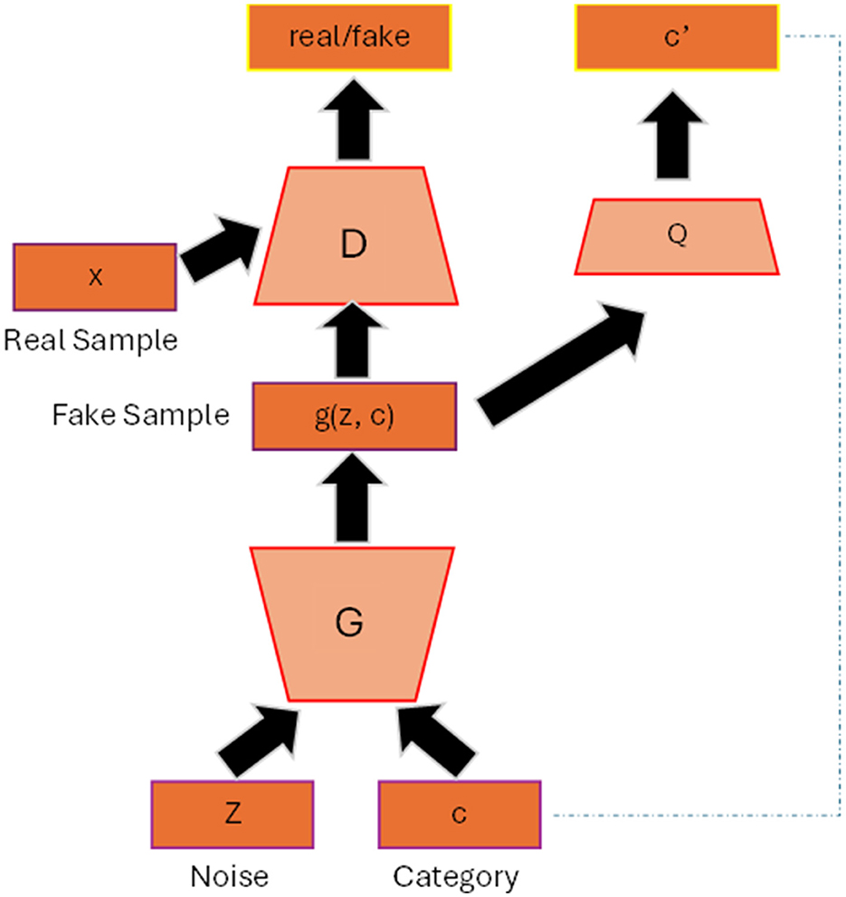
Figure 1. InfoGAN architecture. The data attribute c is added to the input of the generator. The Q classifier uses the generated data from G as input and produces the information distribution c′ that resembles c.

2.3 Conditional GAN

Figure 2 shows the general architecture of conditional GAN (cGAN) (Mirza and Osindero, 2014). By adding the auxiliary information c to the generator and discriminator such as class label, the model can generate data that belongs to that specific label. The conditioned information not only guides the generator to produce high quality synthesis image but also helps to improve the stability of the training process. The loss function will then include the conditioned c as depicted in Equation 4 and Equation 5:

LD=maxD?x~preal(x)[logD(x|c)]      +?x^~pθ(x^|z)[log(1-D(G(z|c)))]    (4) LG=minG?x^~pθ(x^|z)[log(1-D(G(z|c)))]    (5)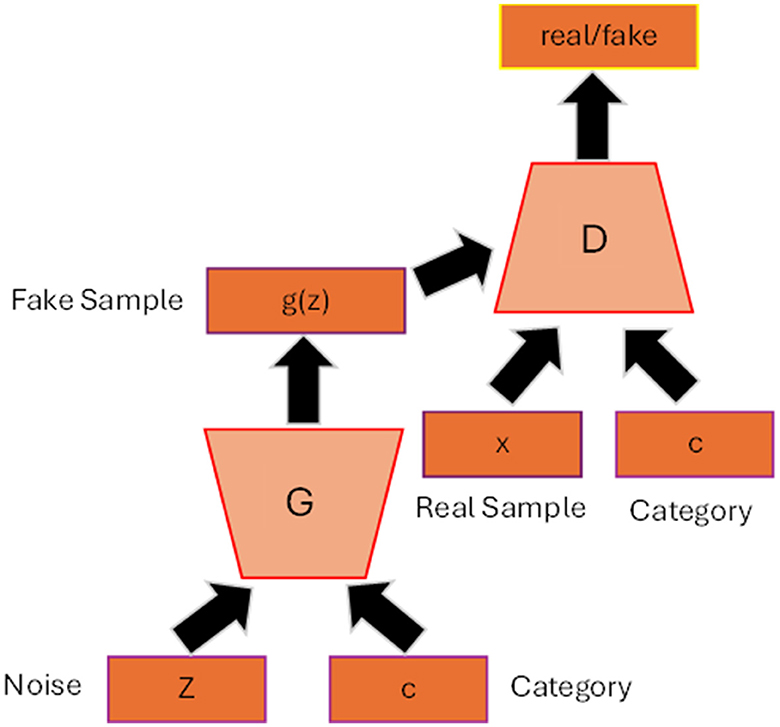

Figure 2. Conditional GAN architecture. The label c is added as input to the generator and discriminator so that the generator can generate synthetic data belonging to that specific label.

2.4 AC-GAN

The auxiliary classifier GAN (AC-GAN) (Odena et al., 2017) is an extension of the cGAN where the discriminator is slightly modified so that it can also provide the prediction of the class label along with the authenticity of the input. In particular, similar to cGAN, the generator will also receive the class label combined with the latent vector as input, while the discriminator is provided with only the images, instead of both the images and class label in cGAN. The discriminator will add one more head that uses softmax activation function to provide the probability for each class label, enabling GAN to performance classification task.

2.5 Wasserstein GAN

Wasserstein GAN (WGAN) (Arjovsky et al., 2017) was proposed to deal with the common issues that often occur when training the GAN model, such as mode collapse or JS divergence. The paper introduces the new distance metric—Earth Moving distance or Wasserstein distance that can be formulated as in Equation 6:

W(ℙr,ℙθ)=sup∥f∥L≤1?x~ℙr[f(x)]-?x~ℙθ[f(x)]    (6)

where f is a 1-Lipschitz function. To solve this equation, we can model f as a neural network and learn the parameters from it. The solution can be shortly summarized as in Equation 7:

maxw∈W?x~ℙr[fw(x)]-?z~pz[fw(gθ(z))]    (7)

Initially, the model used weight clipping technique to satisfy the Lipschitz constraint that may lead to vanishing gradient problem. The paper later introduced a gradient penalty technique to enforce Lipschitz constraint to improve the stability of the training process.

2.6 CycleGAN

CycleGAN (Zhu et al., 2017) is one of the most commonly used models in the generation of medical images due to its capability to perform cross-modality transition, such as synthesizing brain CT images from MRI images. CycleGAN consists of two generators and two discriminators where each generator will receive a set of data from other modality and the data are not necessary to pair with each other. Let us assume that we have data samples x∈X and y∈Y where X, Y are training data for which we want to make a transition and G, F are two generators or two translators that make a mapping: ŷ = G(x) and x^=F(y). If we use the original GAN's loss function to update the model, the generator may be able to generate data in each domain, but it is not sufficient to generate translations of the input data. CycleGAN introduces an additional concept called cycle consistency which states that the transitions between the two translators are bijections, meaning that F(G(x)) = x and G(F(y)) = y. The cycle consistent loss is added to the original loss function as the regularization term as shown in Equation 8:

Lcyc(G,F)=?x~pdata(x)[∥F(G(x))x∥1]                  +?y~pdata(y)[∥G(F(y))-y∥1]    (8)

Figure 3 illustrated the overall architecture of CycleGAN.

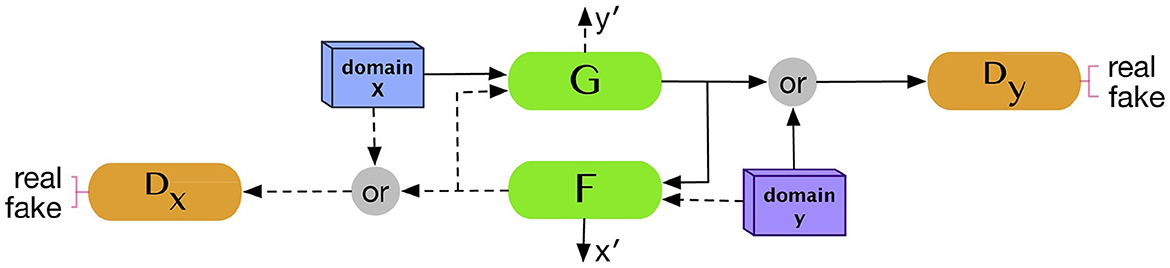
Figure 3. CycleGAN architecture. Two generators and two discriminators are trained in the CycleGAN model. Each generator receives a set of data from the other domain to produce synthetic data from its domain. Reprinted from: Kazeminia et al. (2020). Copyright (2020) with permission from Elsevier.

3 Similarity metrics

The synthetic data must undergo validation against real data to assess the model's effectiveness. Numerous similarity metrics have been developed to evaluate the features of real and synthesized brain networks. This section provides a brief overview of these techniques that have been used in previous literature.

Kullback-Leibler Divergence (KL Divergence) measures the difference between two probability distributions p(x) and q(x) [where p(x) and q(x) are the probability of the data x ∈ X occurring in the real and fake data distribution, respectively]. The formula for KL divergence can be expressed as Equation 9:

KL(p(x)||q(x))=∑x∈Xln p(x)p(x)q(x)    (9)

Maximum Mean Discrepancy (MMD) quantifies distribution differences by measuring the distances between distributions through their respective mean feature embeddings, which can be expressed as Equation 10:

MMD(P,Q)=||?X~P[ϕ(x)]-?Y~Q[ϕ(Y)]||2    (10)

where X and Y are the sample from real distribution P and fake distribution Q, respectively. ϕ is a kernel function that maps X and Y into a higher-dimensional space.

Graph-based global metrics: Transitivity, global efficiency, modularity, density, betweenness centrality, and assortativity (Beauchene et al., 2018) are prevalent metrics employed for quantifying meaningful graph attributes and therefore serving as tools to assess the quality of generated graphs.

4 Applications of GAN for brain disorder classification

One of the most challenging problems in training a deep learning model for brain disorder classification is the small amount of data often causing the model to be overfitted. One possible solution to this problem is using GAN for data augmentation due to its capability to synthesize high-quality images that resemble real MRI data. Many researches have shown that using generated images from GAN can assist the training process and improve the classification performance (Shin et al., 2018). In this work, we will focus on the discussion of the GAN models that utilize synthetic MRI images to assist the classification problem.

Zhou et al. (2021) used both GAN and fully convolutional network (FCN) to generate 3 T MRI images from 1.5 T images in the ADNI dataset to distinguish the brain images of AD patients from those of the healthy group. The goal of the generator is to use 1.5 T data as the input to generate 3 T images (called 3 T*) images with better resolution to improve the classification performance. This method is similar to residual learning, where the model tries to figure out the missing features or the differences between two types of images and the model will add those features to transform 1.5–3T images. The main advantages of this method is that by learning only the residual, we could save a large amount of computational resources and the model could learn the important features more easily.

Training GAN model for the 3D images requires a large amount of data to avoid over-fitting problem. Furthermore, it may not be appropriate for the 2D CNN to be trained on 3D data. Therefore, Kang et al. (2021) suggested to train on multiple 2D slices selected from the coronal axis and then proposed a major voting scheme to obtain best accuracy results. The model was first trained on all the slices with deep convolutional GAN (DCGAN) method (Radford et al., 2015). Then they used transfer learning that froze the few first layers' trainable weights and fine-tuned the weights of the remaining layers on three models: the pretrained DCGAN, VGG16 (Simonyan and Zisserman, 2014) and ResNet50 (He et al., 2016) to select the models that produce the best results. VGG16 and ResNet50 were pretrained on the ImageNet dataset. The results have shown that ensemble learning with three classifiers is more stable and has the highest performance than when training with only one classifier.

Most of the works focus on generating 3-D brain images which demands huge computational resources as well as lacks interpretability. A GAN model that can produce synthetic functional connectivity can be more effective for tackling both of these problems. Geng et al. (2020) proposed a brain functional connectivity generative adversarial network (FC-GAN) that combines variational autoencoder (VAE) and adversarial strategy to generate FC data from the original dataset. The model consists of three components: the encoder took the real data as input to generate the mean and variance of the latent code that follows the normal distribution and use it as a noise vector; the decoder took the noise vector to generate fake data, which is equivalent to the generator component in GAN; and finally the discriminator was designed based on WGAN loss that used Wesserstein distance to calculate the difference between fake and real data. Those three components were jointly connected and trained separately. The whole model was trained in two steps: the first step was trained according to traditional GAN procedure to receive augmented FC data. Then the augmented data was combined with the experimental data and they were fed into the deep neural network (DNN) containing multiple fully connected layers to output the class for each subject. The experimental results on ASD (256 HC and 198 patients with AD), ADHD (272 HC and 215 patients with ADHD), and ASD-ABIDE datasets (829 HC and 660 patients with AD) show the improvement in accuracy when training with DNN alone (87.16, 87.27,and 70.22%, respectively, compared to 85.35, 85.06, and 67.22%, respectively).

GAN with autoencoder was also applied in generating brain connectivity for the classification of multiple sclerosis (MS) (Barile et al., 2021) (Figure 4). However, the output of the encoder will try to resemble the data drawn from the normal distribution instead of the image data. The model demonstrated an improvement of accuracy when training with the generated connectomes than with the original ones, meaning that the model could generate meaningful connections that could help to identify the disease. The model was tested on Multiple Sclerosis (MS) dataset, which included 29 relapsing-remitting and 19 secondary-progressive MS patients, achieving the highest F1-score of 81% compared to only 65.65% without using a data augmentation method. The model also outperformed other data augmentation techniques by margins exceeding over 10% (72.32% for SMOTE and 64.84% for the Random Over Sampling (ROS) method).

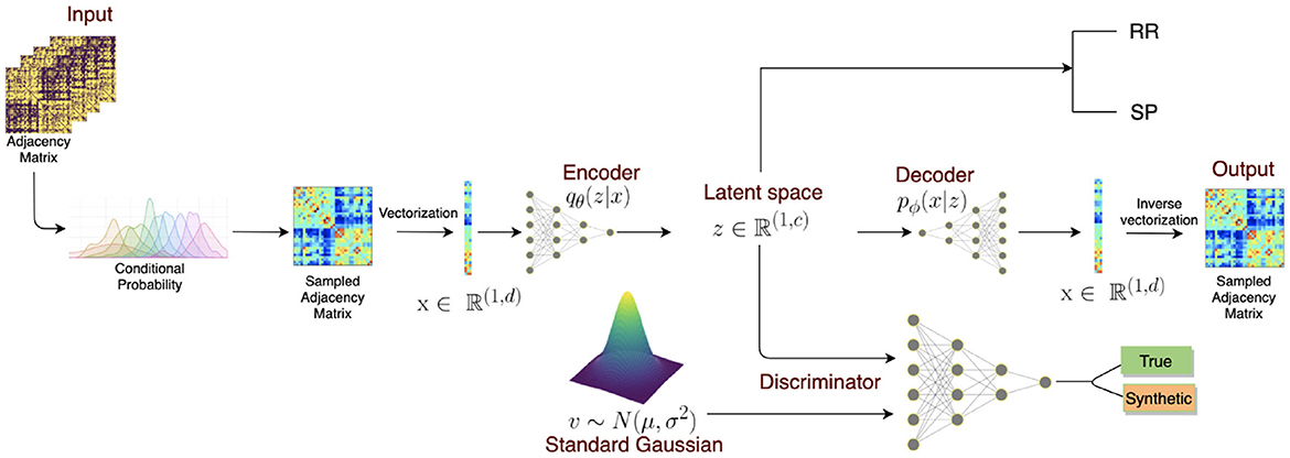
Figure 4. VAE + GAN end-to-end architecture. The model consists of three parts: (1) an encoder transforms the sampled adjacency matrix inputs to a latent lower dimensional representation. (2) The decoder aims to reconstruct the original input from the latent representation z. (3) The discriminator takes both the latent representation and random noise vector as inputs and tries to discriminate these distributions. Once the model is trained, the model can generate synthetic graphs from a standard Gaussian distribution which then can be combined with experimental data for classification. Reprinted from: Barile et al. (2021). Copyright (2021) with permission from Elsevier.

Another FC-based method that also applied a GAN model for the classification of major depressive disorder (MDD) patients from HC was proposed by Zhao et al. (2020). The model implemented a feature mapping technique in GAN, which is a specific method that can increase the efficiency of the training process of the GAN model (Salimans et al., 2016). The feature mapping method changes the way of training the generator where the discriminator will guide the generator to match the features of the intermediate layer of the discriminator. The new objective function for the generator can be defined as Equation 11:

∥Ex~pdataf(x)-EZ~pZ(z)f(G(z))∥22    (11)