the type of gesture, T the number of time samples in a gesture epoch, let P(k) ∈ ℝE×T denote the prototyped response, i.e. the mean EMG signal computed from all epochs of gesture type k, and λ ∈ ℝE×NT be the matrix obtained by concatenating all the epochs of EMG signals from the entire set of gestures. Each spatial filter is optimized to enhance the SSNR of its corresponding gesture type k and represented as a vector w ∈ ℝE×1 defined by Equation (3): w*(k)=argmaxwwTP(k)P(k)TwwTλλTw    (3)

With F ∈ ℕ the parameterizable number of xDAWN spatial filters, let W(k) denote the F selected spatial filters for gesture type k, and W =[W(1), ..., W(k)] ∈ ℝE×KF the aggregation of those spatial filters. Let Xi∈ℝE×T a gesture epoch of index i, the spatially filtered signal of Xi is defined by Zi∈ℝKF×T as in Equation (4):

We define a new matrix Z~i∈ℝ2KF×T by concatenating (i) the filtered averaged trials P(k) for all gesture types k with (ii) the spatially filtered EMG signal Zi as in Equation (5):

Z~i=[W(1)TP(1)...W(k)TP(k)Zi]    (5) 2.4.2.2 Covariance matrices

In the context of EMG classification, covariance matrices capture information about how muscle signals vary together or independently. By identifying patterns and similarities in muscle activity, they provide a discriminative and compressed representation of EMG signals that have the potential to significantly enhance the performance of classification models for gesture recognition.

The set of symmetric n × n real matrices is a n(n + 1)/2-dimensional real vector space ∀n ∈ ℕ, and therefore has a canonical Riemannian manifold structure. Covariance matrices belong to the set of symmetric positive definite matrices which is a convex cone (Moakher, 2005; Sra and Hosseini, 2015). In such a space, the use of Euclidean distances is unsuitable due to fundamental geometric differences. The inherent curvature of Riemannian manifolds results in distances following non-linear paths, which Euclidean distances cannot accurately represent. Therefore specialized metrics or methods are needed to discriminate covariance matrices of EMG signals.

2.4.2.3 Tangent space projection

In addressing this challenge, two approaches have emerged. The first involves adapting the classification models (Barachant et al., 2013; Huang and Gool, 2017), or their optimization algorithms (Kochurov et al., 2020), to accommodate the specificities of Riemannian manifolds. The second approach focuses on projecting covariance matrices from the Riemannian manifold into a specific tangent space where, given an appropriate choice of the reference point for tangent space computation, the Euclidean distance represents a good approximation of the Riemannian distance on the manifold itself (Congedo et al., 2013). The latter is particularly interesting as it enables the direct application of common classification algorithms to projected covariance matrices without significant performance loss.

Let Σref denote the reference point on the Riemannian manifold M where the tangent plane is computed. As showed in Tuzel et al. (2008), the Fréchet mean of the set of covariance matrices is the Σref where the projection onto the tangent space provides the better local approximation of the manifold. On this Riemannian manifold, every covariance matrices Σ ∈ M can be projected onto the tangent space computed at the reference point Σref (Pennec et al., 2006). With E the number of electrodes, 1E the matrix of ones and IE the identity matrix, both of size E×E, the projection operator ?Σref is defined by Barachant et al. (2013) as to map every matrix Σ to the vector representation of the upper triangular submatrix of 2(1E1ET-IE)Φ(Σ). With log the matrix logarithm, and logΣref(Σ) the matrix logarithm of Σ with respect to Σref, Φ(Σ) is defined in Equation (6).

Φ(Σ)=logΣref(Σ)=Σref1/2log(Σref-1/2ΣΣref-1/2)Σref1/2    (6) 2.4.2.4 Implementation of the pipelines

In this work, we evaluate the performance of two classification pipelines based on covariance matrices and Riemannian geometry.

The first pipeline called Covariance estimates covariance matrices Σi∈ℝE×E from Xi∈ℝE×T, with Xi the raw EMG signal of the gesture epoch of index i with E[Xi] = 0 as in Equation (7).

The second pipeline called xDAWN Covariance estimates the covariance matrices Σi∈ℝ2KF×2KF from Z~i∈ℝ2KF×T, with Zi the xDAWN-filtered EMG signal of the gesture epoch of index i as in Equation (8).

Let Ωi = ?Σref(Σi), be the generic feature vector obtained after projecting the covariance matrix Σi, estimated from either the raw or xDAWN-filtered EMG signal, onto the tangent space. The final classifier, common to both pipelines, is a logistic regression (LR) as defined in Equation (2).

The parameters estimated during the training of the classification pipelines are (i) the spatial filters W (only in the xDAWN Covariance pipeline), (ii) the reference point Σref and (iii) ω0, ω respectively the intercept and the normal vector of the hyperplane.

The covariance matrices were computed with the well-conditioned estimator OAS (Chen et al., 2010). The estimation and application of xDAWN spatial filters, as well as the computation of Σref, and the projection operator to the tangent space ?Σref(Σi) were implemented in the pyRiemann (Barachant et al., 2023) Python library. The multiclass logistic regression trained to classify the gesture type used the one-vs-rest training scheme with L2 penalty and liblinear solver, as implemented in Pedregosa et al. (2011).

2.4.3 Pipeline based on convolutional neural networks 2.4.3.1 Network architecture

Building on the success of the perceptron (Rosenblatt, 1958) and the multilayer perceptron (Amari, 1967) (MLP) to learn complex high-dimensional patterns, new hierarchical network architectures (Fukushima, 1980) were developed inspired by previous work on the neural receptive fields of the cat visual cortex (Hubel and Wiesel, 1959). The convolutional neural network (Lecun et al., 1998) (CNN) is a biologically-inspired variant of the MLP which hierarchically extracts high-level spatial or temporal patterns using convolution operators. As of today, CNN are considered one of the state-of-the-art model for image classification and segmentation due to their first-class performance coupled with limited preprocessing requirements. These performances recently led to a growing interest from the scientific community to use CNN for the classification of physiological signals such as EEG (Dai et al., 2019) or EMG (Hioki and Kawasaki, 2009; Karnam et al., 2022).

A CNN typically consists of two main parts which play different roles in the network's architecture: the convolutional blocks and the fully-connected layers.

The convolutional blocks are responsible for feature extraction from the input data and are especially well-suited for tasks that involve grid-like data, such as images, or spatiotemporal data such as EMG. Multiple convolutional blocks are stacked to detect hierarchical features, from simple features in the early layers to more complex features in deeper layers. Each convolutional block typically comprises at least the following layers:

• A convolutional layer composed of a set of learnable n-dimensional kernels acting as pattern filters. Each kernel is convolved across the whole input layer to produce an activation map. Formally, in the context of a one-dimensional convolution, let x ∈ ℝN be a one-dimensional input, e.g., an EEG signal from a specific electrode, h ∈ ℝM be a one-dimensional kernel. The output of the one-dimensional convolution of xn through hm is given by Equation (9).

(x*h)n=∑m=0M-1hmxn-m   ∀n=0,...,N-1    (9)

• A pooling layer which downsamples feature maps and reduces the spatial dimensions by locally applying the non-linear max or mean function.

• A regularization layer, which enhances the model's generalization and training stability by using techniques such as batch normalization or dropout. These techniques help mitigate issues like overfitting and internal covariate shift (in the case of batch normalization).

The fully-connected layers (also denoted hidden-layers) extract global patterns by combining high-level activation maps hierarchically produced by the convolutional blocks in order to make a final classification. The output of each neuron from a fully-connected layer consists of a linear combination of its inputs followed by an activation function σ. An activation function is a differentiable, non-linear function applied to the output of each neuron in order to create a non-linear decision boundary from a linear combination of inputs and weights. The use of non-linear activation functions between each hidden layer enables the separation of input vectors that are not linearly separable (Cybenko, 1989). Formally, let ℓ ∈ ℕ>0 denote the index of some hidden layer, n(ℓ)∈ℕ>0 be the number of neurons in hidden layer ℓ, zv(ℓ)∈ℝ ∀v ∈ be the output of the vth neuron of layer ℓ, wkv(ℓ)∈ℝ be the weight of the edge connecting the kth neuron of layer ℓ−1 to the vth neuron of layer ℓ, z0(ℓ)∈ℝ be the bias of layer ℓ and σ(ℓ) be the non-linear activation function of layer ℓ, the output of the vth neuron of layer ℓ is given in Equation (10).

zv(ℓ)=σ(ℓ)(∑k=1n(ℓ-1)wkv(ℓ) zk(ℓ-1)+w0v(ℓ) z0(ℓ-1))    (10)

The final layer of the fully-connected layers is referred to as the output layer. In a classification task, the output layer typically contains one neuron per class, with the output values representing the class probabilities computed using the Softmax activation function (Bridle, 1990).

The choice of weights initialization and non-linear activation function in convolution kernels and fully-connected layers is paramount to avoid undesirable effects such as the vanishing or exploding gradient problems (Bengio et al., 1994) when training deep architectures. In this work, we used the rectified linear unit (Nair and Hinton, 2010) activation function and weights were initialized following the Glorot (Glorot and Bengio, 2010) uniform distribution. Formally, let n(ℓ)∈ℕ>0 be the number of neurons in hidden layer ℓ, w(ℓ) ∈ ℝn(ℓ−1)×n(ℓ) be the weights vector of layer ℓ, the initialization of w(ℓ) following the Glorot uniform distribution is defined by Equation (11).

wij(ℓ)∽ U(-6n(ℓ-1)+n(ℓ) , 6n(ℓ-1)+n(ℓ))    (11) 2.4.3.2 Proposed CNN architecture

After trying multiple network architectures, the following architecture achieved the best cross-validated performance both for phasic and tonic EMG:

• A linear temporal convolution with 128 filters of shape (1 × 16).

• A spatial convolution with 16 filters of shape (8 × 1) followed by a batch normalization layer, a ReLU non-linear activation function, a mean pooling layer of shape (1 × 4) and a spatial dropout layer.

• A temporal convolution with 128 filters of shape (1 × 16) followed by a batch normalization layer, a ReLU non-linear activation function, a mean pooling layer of shape (1 × 4) and a spatial dropout layer.

• Two fully-connected layers of 128 neurons each followed by a ReLU non-linear activation function.

• A fully-connected layer of four neurons (corresponding to the 4 different gestures) followed by a softmax activation function.

2.4.3.3 Network training procedure

The training procedure of the CNN relies on the backpropagation algorithm (Rumelhart et al., 1986), which vanilla implementation is based on stochastic gradient descent. The backpropagation algorithm iteratively updates the set of trainable parameters of the CNN by using the chain rule to compute the partial derivatives of the loss function with respect to those parameters. With θt the parameters at time step t, α the fixed learning rate, and ∇f(θt) the gradient of the loss function with respect to θt. The updated parameters are defined by Equation (12).

θt+1=θt-α∇f(θt)    (12)

In this work, we use the Adam optimization algorithm (Kingma and Ba, 2014) that enhances the traditional stochastic gradient descent by accelerating its convergence using adaptive learning rates for each parameter, incorporating momentum and adaptive step sizes. The starting learning used in the proposed architecture is 0.005.

2.5 Validation methodology

To validate the classification results, we evaluate the generalization capabilities of the estimation pipelines in three distinct configurations illustrated in Figure 6: the intra-subjects, inter-sessions, and inter-subjects.

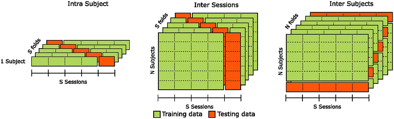
Figure 6. Illustration of the cross-validation methods used for intra-subjects, inter-sessions, and inter-subjects analyses of classification results.

In the intra-subjects configuration, we assess the estimator's robustness by training it on 80% of the training set and evaluating it on the remaining 20%, representing a “holdout" portion of the data that the model has never seen. To prevent potential bias due to specificities in portions of the training set or uneven class representation in the validation set, we use a stratified five-fold cross-validation and report the mean accuracy across all folds. We repeat this procedure for each participant, and the final estimator performance is computed as the mean accuracy across all individual cross-validated estimators. The intra-subjects configuration provides insights into an estimator's capacity to generalize to new, unseen data from the same participant. However, it does not provide any information on the estimator's ability to generalize to data from different participants.

In the inter-sessions configuration, we assess the estimator's robustness by training it on four out of the five sessions of all participants and evaluating it on the “holdout” sessions that the model has never seen. To prevent bias due to potential sessions' specificities, we use a Leave-One-Group-Out cross-validation, with each “group” corresponding to a session. The final estimator performance is computed as the mean accuracy across all five cross-validated estimators. The inter-sessions configuration provides insights into an estimator's capacity to generalize to unseen data from new sessions of the same participants. However, similarly to the intra-subjects configuration, it does not provide any information on the estimator's ability to generalize to data from new unseen participants.

In the inter-subjects configuration, we assess the estimator's robustness by training it using data from all but one participants and evaluating it on the “holdout" participant that the model has never seen. To prevent bias due to potential participants' specificities, we use a Leave-One-Subject-Out cross-validation. The final estimator performance is computed as the mean accuracy across all n cross-validated estimators, with n being the number of participants. Contrary to intra-subjects and inter-sessions configurations, the inter-subjects configuration provides insights into an estimator's capacity to generalize to unseen data from new participants.

2.6 Physiological decomposition of the EMG signal

As previously introduced, the EMG signal can be categorized as phasic (during the production of movement) or tonic, during steady postures. Defining the precise boundary between these categories can be challenging. In this study, we decided to distinguish between tonic and phasic activity by choosing a specific time period after a careful visual inspection of the EMG signals. Another interesting perspective is to consider EMG signals as a combination of two commands: the “move command” that controls the movement of the limb to the target posture and influences primarily phasic activity, and the “hold command” that maintains the limb at the target posture and influences tonic activity. The raw EMG signal represents the sum of both commands.

How to decompose the signal into “move” and “hold” commands is not completely understood yet. Albert et al. (2020) have hypothesized that, for hand gestures, the instantaneous amplitude of the “hold” command of a specific posture is defined by the integral of the instantaneous amplitude of the “move” command that led to this posture. The instantaneous amplitude of the EMG signal (also referred to as the “envelope” of the signal) represents the strength of the muscle activation at any point in time, regardless of the phase of the signal.

We compute the envelope of the EMG signal by initially performing full-wave rectification on the analytic signal derived from the application of the Hilbert transform (Boashash, 1992; Myers et al., 2003). Formally, for a given signal x(t), we have its instantaneous amplitude a(t)=x2(t)+xh2(t), where xh(t), the Hilbert transform of x(t), is computed using the formula in Equation (13).

xh(t)=p.v.∫-∞+∞x(t-τ)πτdτ    (13)

where p.v. denotes the Cauchy principal value of the integral (Boashash, 1992). Finally, we apply low-pass filtering with a 20 Hz cutoff frequency to smooth the resulting envelope.

Let us note HT, the instantaneous amplitude of the hold command at time T, and MT the instantaneous amplitude of the move command at time T. The mathematical integration of physiological signals described by Albert et al. (2020) is as follows in Equation (14).

In the envelope of a discrete recorded EMG signal S, the value at each time step T is equal to the sum of the two commands: ST = MT+HT. To estimate the decomposition of the signal's envelope into M and H, we use the iteration defined in Equation (15).

{MT=ST−HT−1HT=HT−1+MTf    (15)

In these formulas, f is the sampling frequency. Initially, H0 and M0 are set to 0 and T = 0 should correspond to the beginning of the move command. After decomposing the signal, we obtain two separate envelopes, that can be used as input of a machine learning model, similarly to the raw signal.

We note that the mathematical integration method is not the only hypothesis for decomposing the EMG signal into its fundamental components. For example, Flanders and Soechting (1990) described a more complex analysis based on principal components scaled down with movement time.

3 Results 3.1 EMG visualization during guided gestures

We aim to gain a comprehensive understanding of the EMG behavior during guided gestures. To achieve this, we present an analysis of the median and quartile values of the envelope of the EMG signal (as presented in Section 2.6) during the execution of the four distinct gestures. We also remove the baseline activity associated with the resting pose, thereby allowing us to highlight the dynamic aspects of muscle activity during the guided gestures. As shown in Figure 7, the gestures involve three phases. First, when the subject transitions from the resting pose to the target pose, we observe a short and strong increase in muscle activity. After that, a residual activity is observed during the hold of the posture, indicating that the muscles are still more engaged than during the resting posture. Finally, a second peak of activity appears when going back to the resting pose. The plots of different EMG channels in Figure 7 indicate a clear difference between the roles of each muscle. Those more active during the first phase might correspond to flexor muscles, while those more active during the last phase should be extensor muscles.

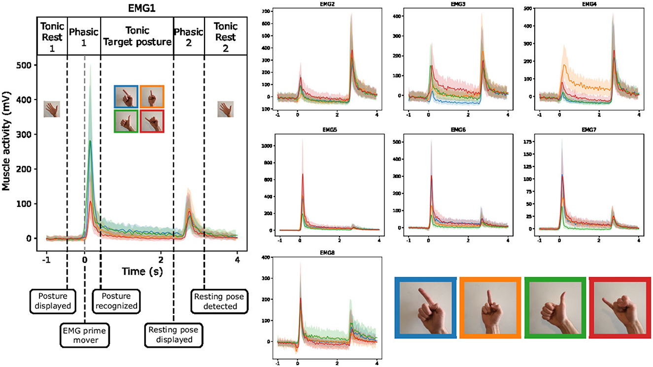
Figure 7. Envelope (median and quartiles) of the EMG signal during the realization of predefined gestures by one subject (right hand of the subject 4). The signals are aligned at the prime mover event.

Figure 7 suggests that discriminating between the recorded gestures executed by a single participant's hand should be a manageable task, given the distinctive EMG patterns exhibited by the different gestures. Especially, when looking at the EMG3 channel, we observe strong differences between gestures during both the first gesture phasic and the tonic phase of the target posture.

To better understand inter-subjects variability, we use a similar figure that highlights the behavior of the EMG1 channel on the two hands of different participants. We observe from Figure 8 that the overall amplitude of the signal changes significantly across the subjects even with normalization applied from MVC. Moreover, regardless of the signal amplitude, the shape of the signal during the different gestures is also subject-dependent, and often even changes between the left and right hand of the same person. These differences help to understand the lower efficiency of inter-subject estimation models that are commonly obtained in the literature.

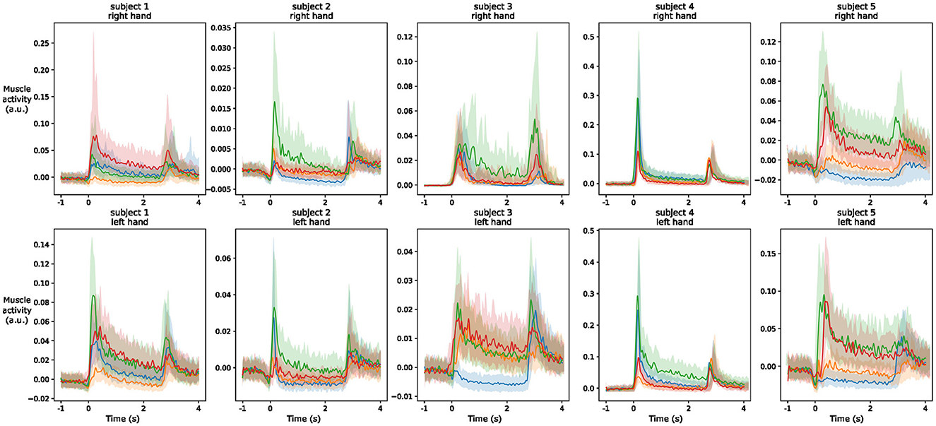
Figure 8. Envelope (median and quartiles) of the EMG signal of electrode 1 during the realization of predefined gestures by different subjects. The signals are aligned at the prime mover event and normalized using division by the maximum value of the signal during maximum voluntary contraction of the muscles. The colors of the four gestures are similar to those in Figure 7.

3.2 Classification of guided gestures

The main results of the classifications pipelines using both the phasic and tonic components of EMG signals in intra-subject, inter-sessions, and inter-subjects configurations were illustrated by confusion matrices, receiver operating characteristic (ROC) curves (with the corresponding AUC values), and average ranks of the classification pipelines. For the clarity of illustration, we aggregated the results from the four classification pipelines by computing the average of their predictions and denoted this new model Voting ensemble. The aggregated performances of the four classification pipelines using the phasic and tonic components are illustrated in Figures 9, 10 respectively. The individual performances of each classification pipeline are illustrated in Figure 11. Statistical differences between classification pipeline performances were performed with a post-hoc Nemenyi test (Demšar, 2006) using the Autorank Python library (Herbold, 2020).

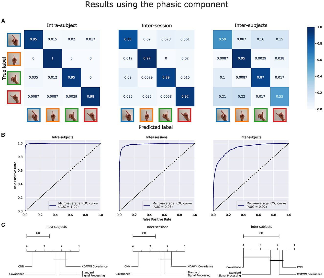
Figure 9. Results of the voting ensemble of the four classification pipelines using the phasic component of the EMG signals in intra-subject, inter-sessions, and inter-subjects configurations. (A) Confusion matrices. (B) ROC curves. (C) Average rank of the corresponding classifiers (the lower, the better). Classifiers that are not significantly different are connected by a black line [at p = 0.05 found by a Nemenyi test (Demšar, 2006)]. The critical distance (CD) indicates when classifiers are considered statistically different.

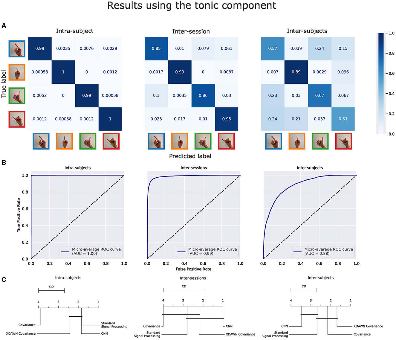
Figure 10. Results of the voting ensemble of the four classification pipelines using the tonic component of the EMG signals in intra-subject, inter-sessions, and inter-subjects configurations. (A) Confusion matrices. (B) ROC curves. (C) Average rank of the corresponding classifiers (the lower, the better). Classifiers that are not significantly different are connected by a black line [at p = 0.05 found by a Nemenyi test (Demšar, 2006)]. The critical distance (CD) indicates when classifiers are considered statistically different.

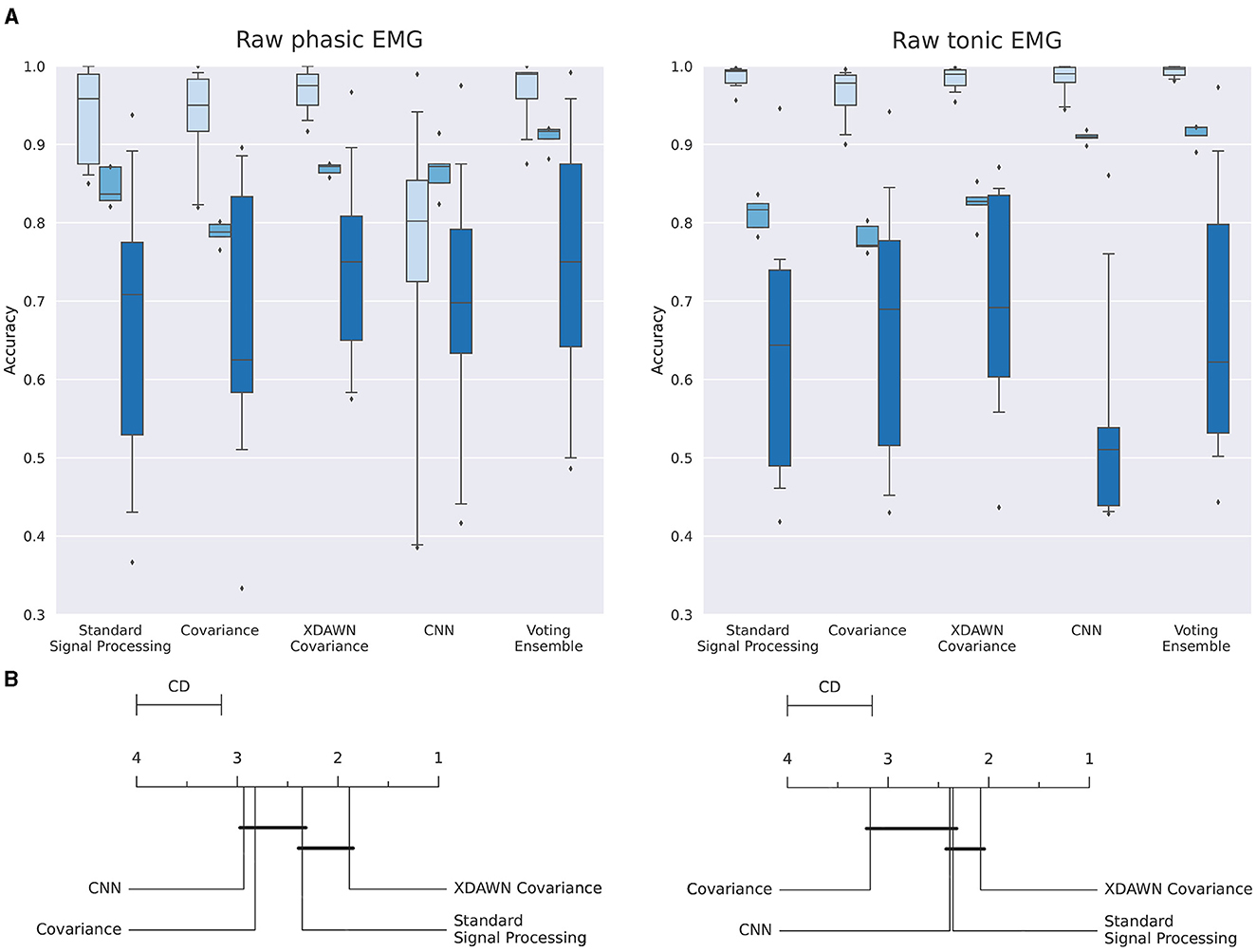
Figure 11. (A) Boxplots illustrating the multiclass classification accuracy of the four classification pipelines and the Voting ensemble using the phasic or tonic components of the EMG signals in intra-subject (light blue), inter-sessions (medium blue), and inter-subjects (dark blue) configurations. (B) Average rank of the corresponding classifiers for the three configurations (the lower, the better). Classifiers that are not significantly different are connected by a black line [at p = 0.05 found by a Nemenyi test (Demšar, 2006)]. The critical distance (CD) indicates when classifiers are considered statistically different.

Additionally, to assess the performances of the four classification pipelines using high-quality EMG signals, we excluded the sessions with low-quality EMG (as explained in Section 2.3) from the dataset used to generate the results of the present section.

3.2.1 Classification results using the phasic component of the EMG signals

Figure 9 illustrates these performance metrics computed on the Voting ensemble in intra-subject, inter-sessions, and inter-subjects configurations using only the phasic component of the EMG signals. The Voting ensemble model achieved an accuracy of 96.7%, 90.9%, and 73.9%, along with AUC values of 1.0, 0.98, and 0.92, in the intra-subjects, inter-sessions, and inter-subjects configurations, respectively. The confusion matrices in Figure 9A show a balanced recognition accuracy in the intra-subjects configuration but not in the inter-subjects configuration, where gestures involving the index and pinky fingers were notably less well classified than those involving the thumb and middle fingers. The average ranks illustrated in Figure 9C show that the xDAWN Covariance pipeline achieved the highest rank among the four classification pipelines in the intra-subjects and inter-sessions configurations. However, Figure 9C did not show a significant statistical difference between the performances of xDAWN Covariance and the other best-performing classification pipelines. Interestingly, while the CNN pipeline exhibited significantly lower performance than the other classification pipelines in intra-subjects (likely due to the limited amount of data from the small number of gesture repetitions per subject) and inter-sessions configurations, it ranked highest in the inter-subjects configuration, slightly ahead of the xDAWN Covariance pipeline.

3.2.2 Classification results using the tonic component of the EMG signals

Figure 10 illustrates the same performance metrics as Figure 9 computed on the Voting ensemble in intra-subject, inter-sessions, and inter-subjects configurations but using only the tonic component of the EMG signals. The Voting ensemble model achieved an accuracy of 99.3%, 91.1%, and 66.7%, along with AUC values of 1.0, 0.99, and 0.88, in the intra-subjects, inter-sessions, and inter-subjects configurations, respectively. Similarly to the confusion matrices from the phasic component, the confusion matrices from the tonic components in Figure 9A show a balanced recognition accuracy in the intra-subjects configuration but not in the inter-subjects configuration, where, gestures involving the index and pinky fingers were notably less well classified than those involving the thumb and middle fingers. The average ranks illustrated in Figure 9C did not highlight a particular significant statistical difference between the performances of the four classification pipelines using the tonic component of the EMG signals. Here, the CNN pipeline in the intra-subjects configuration exhibits significantly better performance using the tonic component.

3.2.3 Summary of the classification results

The individual performances of each classification pipeline using both the phasic and tonic components of EMG signals in intra-subject, inter-sessions, and inter-subjects configurations are summarized and illustrated in Figure 11.

Figure 11A (left, right) illustrate the individual performances using respectively the phasic and the tonic components of the EMG signals in intra-subject, inter-sessions, and inter-subjects configurations.

In Figure 11A (left), in the intra-subjects, inter-sessions, and inter-subjects configurations, respectively, the classification pipeline bas