Overview of the hifiasm-meta binning algorithm

In the hifiasm-meta assembly graph (Fig. 1A), we noticed circular unresolved subgraphs which are likely due to high strain diversity or shared homology around HGT. Checking the CheckM1 report, we found these circles often corresponded to real bacterial genomes. The observation inspired us to develop an algorithm to enumerate circular paths in the assembly graph. More exactly, we perform a series of depth-first search (DFS) traversals on the assembly graph in attempt to find circular paths of roughly 500 kb or longer. Some circular paths found this way may come from one subgraph and may be redundant. We apply the Mash MinHash-based algorithm [18] to estimate the pairwise distances between circular paths and remove a circular path if it is \(\ge\)95% similar to another circular path. This procedure gives us a list of non-redundant circular paths.

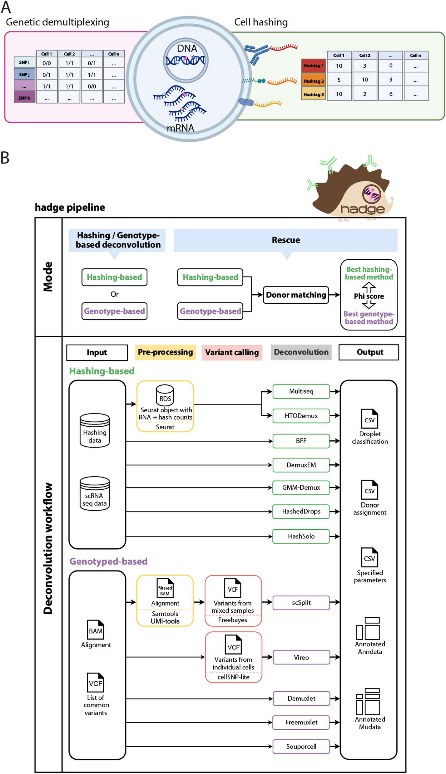
Fig. 1

Showcases of when the circle rescue works well and not well. A The top row shows visualization of three subgraphs from hifiasm-meta primary assemblies, with contigs colored randomly [19]. The bottom row shows the circles (i.e., putative MAGs) rescued by the heuristics, with contigs of each circle colored the same. Contigs that do not belong to any rescued circle are colored gray. These circles were near-complete MAGs based on CheckM1. B The heuristics does not work well in subgraphs or regions like this one. In this particular example, the contigs had very low coverages

Circle rescue cannot group disconnected contigs and thus does not replace classical binning. To provide a smoother user experience, we also implemented a native binning algorithm tightly integrated in hifiasm-meta. At this step, we ignore circular contigs or linear contigs that are on non-redundant circular paths. For each remaining contig, we compute the read coverage in the logarithm scale, count the occurrences of canonical 5-mers and then create a feature matrix of size \(N\times (512+1)\), where N is the number of considered contigs, 512 is the number of canonical 5-mers, and the last dimension is for read coverage. We normalize each column in the matrix by Z-score, embed it to a 2-dimensional space with t-SNE, and extract contig bins in the embedded space using a small radius as follows. We seed a cluster from the longest non-circular contigs to the shortest. For each seed, we try to find a circle with diameter D on the t-SNE plane such that it contains the seed and all other contigs that are \(\le D\) away from the seed. These contigs are called neighbors. If found, the seed and neighbors are put into a bin and marked as used; otherwise, we test whether the circle centered at the seed with diameter \(1.6\times D\) contains all neighbors and create a bin on success. When both attempts fail, we record the seed as a single-contig bin if it is longer than 500 Kb; otherwise, we do nothing. Finally, we merge the resultant bins with circular contigs and non-redundant circular paths to generate the final results.

We call the algorithm above as hmBin in this article. Similar to vamb, hmBin only uses information from the metagenome reads without using marker genes or relying on known reference bacterial genomes. Nonetheless, hmBin still has a few hyperparameters such as the minimum length of circular paths, the Mash similarity, and the radius used for defining t-SNE clusters. During the development of hmBin, we explored different thresholds and found the binning results are generally insensitive to these thresholds on our datasets (“Methods”). We also tried to use UMAP for clustering. The result was slightly worse than the t-SNE clustering.

The circle rescue heuristic also works with mdBG [20] assembly graphs and can recover a third to a fourth of near-complete MAGs found by hifiasm-meta in tested samples. However, mdBG does not correct insertion/deletion sequencing errors in homopolymers which often interrupt open reading frames and lead to low CheckM1 completeness. We thus did not evaluate mdBG results. MetaFlye does not produce an assembly graph for contigs. It instead generates a repeat graph which, unlike string graphs used by hifiasm-meta, may reuse a unitig in multiple contigs. Our circle finding algorithm only traverses each unitig or contig once and does not work with metaFlye assembly graphs. In theory, it is possible to adapt our algorithm for repeat graphs. However, metaFlye assembly graphs more often look like the one in Fig. 1B. We would not be able to get good results anyway.

Fig. 2

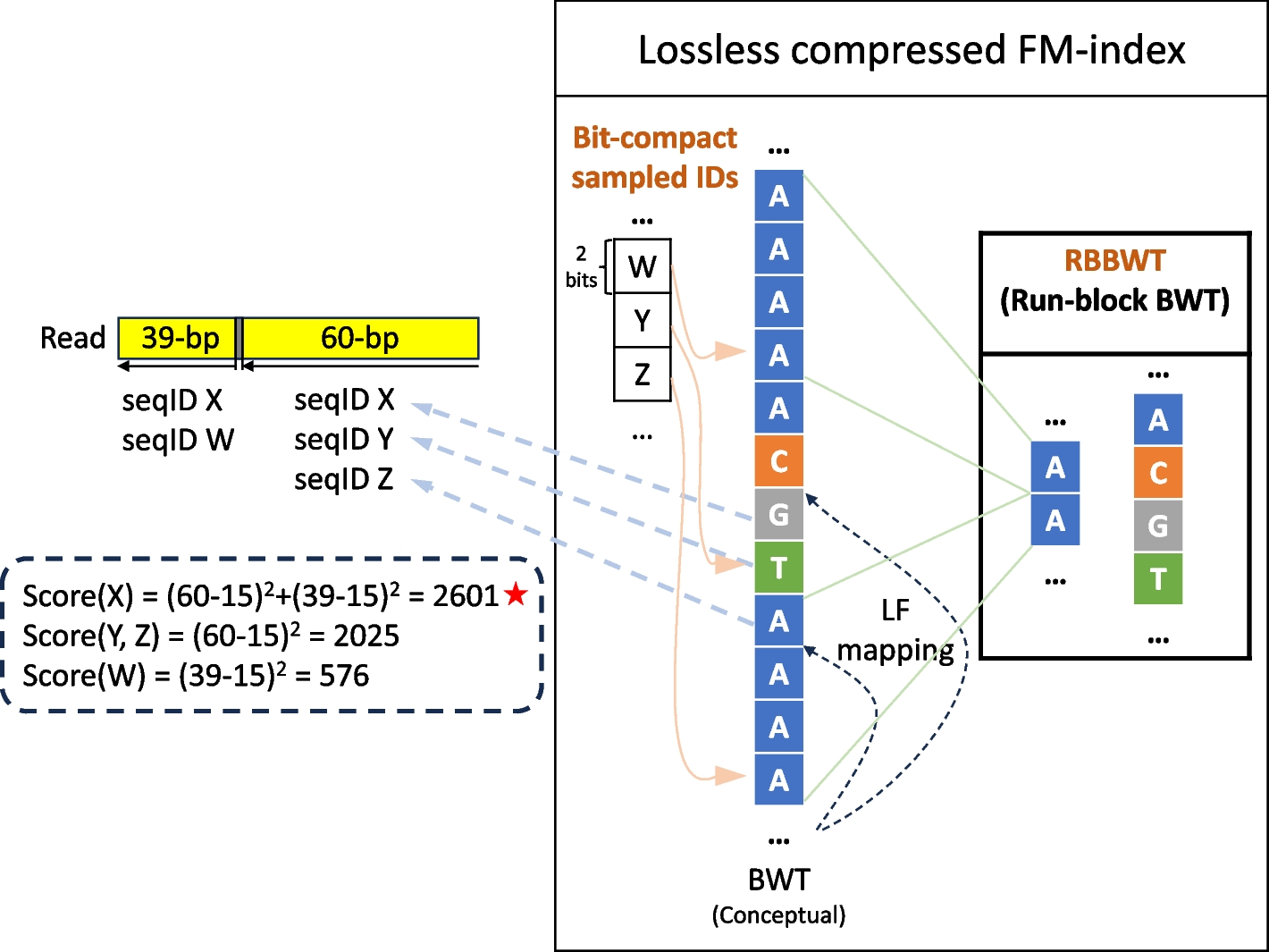
Sankey plot showing flow of reads and contigs of sheep-gut-1b. Left: reads to contigs, categorized by contig length. Middle: contigs to binning categories (from top to bottom, “C” for \(\ge 1\)Mb circular contigs; “PF” for circular path rescue; “scBin: single contig bin; “mcBin” for multi-contig bin; dismissed: unused by binning). Right: MAGs quality categories. Group heights are normalized by counts, except the left-most side which is normalized by base pairs. For the visualization purpose, the height of “dismissed” and the height of “failed” are not proprotional to the counts

Understanding the behavior of the hifiasm-meta binning algorithm

We collected 19 HiFi datasets (Additional files 1 and 2: Tables S1 and S2) and evaluated the quality of MAGs with CheckM1 [4]. Following previous work [21,22,23], we use the following criteria to evaluate MAGs. “Near-complete” means \(\ge 90\%\) completeness and \(< 5\%\) contamination. “High-quality” means \(\ge 70\%\) completeness, \(< 10\%\) contamination but does not qualify for near-complete. “Medium-quality” means \(\ge 50\%\) completeness, \(\ge 50\) quality score but does not qualify for the above two where the quality score of a MAG is defined as “\(\textrm-5\times \textrm\).” All other MAGs are referred to as failed-quality. The categories never refer to the original MiMAG definition, with or without being suffixed by “MAG,” e.g., “HQ” means the high-quality category or the high-quality MAGs under our definition.

Fig. 3

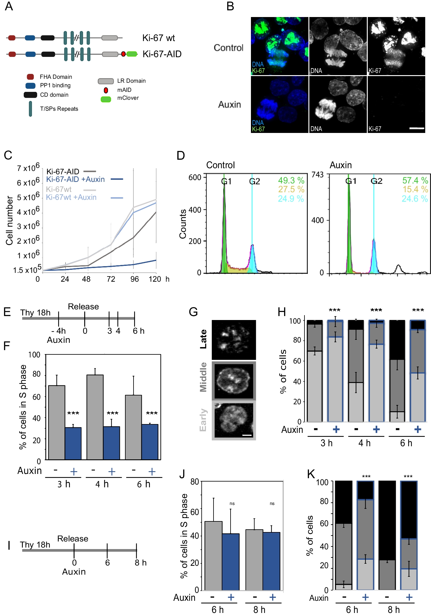
Clustering near-complete MAGs of sheep-gut-1b. The middle-left dense darker square represents Archaea. Mash distance more than 30% are shown as 30%

Figure 2 shows the flow of data when we assembled the sheep-gut-1b dataset with hifiasm-meta and evaluated the results with CheckM1. Notably, a small fraction of circular contigs are not considered near-complete. They may come from underrepresented clades in the CheckM1 data as we found earlier [7]. On sheep-gut-1b, hmBin recovered tens of circular contigs that are considered near-complete by CheckM1 (Fig. 3).

Optimizing other binning algorithms for hifiasm-meta assembly

We additionally applied four other binning algorithms to our datasets, including Vamb [24], MetaBAT2 [25], GraphMB [10], and SemiBin1 [26]. They use different information and distinct algorithms. Vamb only considers coverage and tetranucleotide profiles for binning. MetaBAT2, possibly the most widely used binning algorithm, additionally trains hyperparameters on existing bacterial genomes. GraphMB takes graph topology into account with a Graph Neural Network. SemiBin1 is special in that it uses single-copy marker genes to guide binning, the same information CheckM1 uses to evaluate MAGs. It may be biased to known species and will be unfairly favored by CheckM1. GraphMB can optionally use single-copy marker genes as well. We did not evaluate that mode. We also note that some binners, such as vamb, are optimized for jointly binning multiple samples and may underperform given a single sample.

Fig. 4

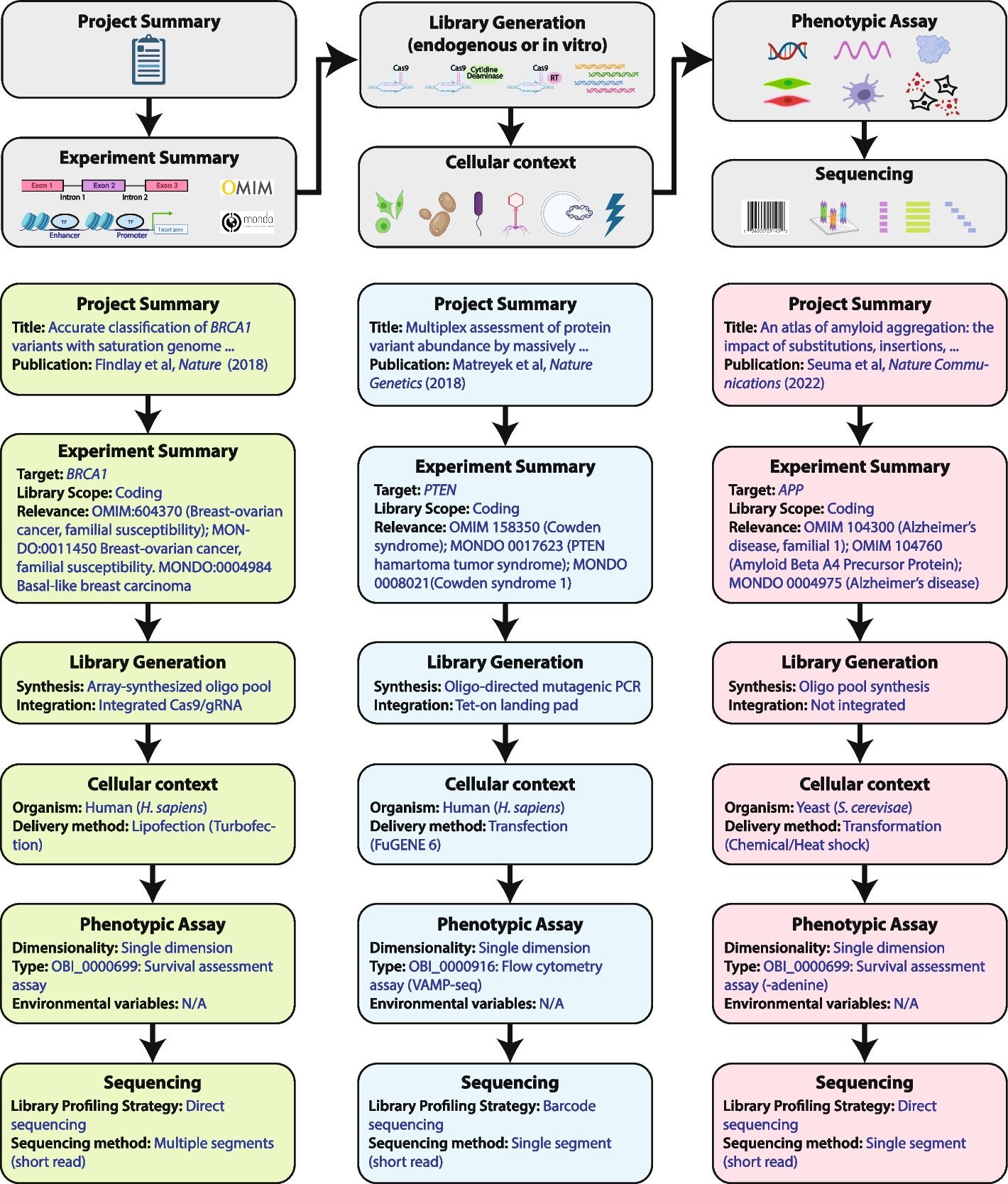
Effect of post-processing and circle rescue on binning quality. A Number of additional near-complete MAGs recovered by putting \(\ge\) 1 Mb circular contigs to separate bins. B Number of additional near-complete MAGs recovered by the hifiasm-meta circle rescue heuristic

As hifiasm-meta may assemble strains of the same species into separate contigs, Vamb, MetaBAT2, and GraphMB may group these contigs and result in complete but highly contaminated bins. To address this issue, we post-process the bins from these binners by putting \(\ge\) 1 Mb circular contigs into separate single-contig bins. Figure 4A shows the effect of putting circular contigs into separate bins. This post-processing step greatly increases the number of near-complete MAGs for the three binners. The improvement is especially notable for the two sheep gut datasets. This step does not help SemiBin1, probably because SemiBin1 can use single-copy marker genes to identify this problem while binning.

Meanwhile, as the hifiasm-meta circle rescue heuristic and traditional binners use different information for binning, the circular paths hifiasm-meta identifies may not always be captured by post-processed bins. We thus additionally merge the circular paths with post-processed bins as follows. For a bin found by a traditional binner of 0.5–10 Mb in size, we discard it as a redundancy if the bin has > 1 Mb sequences or > 10 contigs shared with a rescued circular path. We then combine circular contigs, rescued circles and the remaining bins to produce the final binning results.

Across all the tested datasets, 74 near-complete MetaBAT2 bins were discarded by the procedure above. Sixty-four of them have < 1% mash distance to rescued circles (52 of them < 0.1%). In 61 out of the 64 cases, rescued circles were better than the rejected MetaBAT2 bins in terms of equal or better CheckM1 completeness and contamination. In the remaining three cases, the CheckM1 report on the rescued circles are all close to the report on the MetaBAT2 MAGs (100.0/0.0%, 99.33/1.34% and 90.7/0.94% for MetaBAT2 MAGs, and 98.8/0.48%, 97.32/1.34% and 99.06/2.96% for rescued circles, respectively).

Conversely, 79 out of the 193 near-complete rescued circles were not within 5% mash distance from any near-complete MetaBAT2 bins. Our circle rescue strategy found additional near-complete MAGs on top of MetaBAT2. It also improved Vamb, GraphMB, and SemiBin1 (Fig. 4B), suggesting our strategy captures additional information missed by other binners.

On the binning performance, the integrated hifiasm-meta binning algorithm, hmBin, finds more near-complete MAGs than the raw output of MetaBAT2, Vamb, and GraphMB (Table 1; Additional files 3 and 6: Tables S3 and S6). It is broadly comparable to optimized Vamb and GraphMB and rivals MetaBAT2 only with the post-processing step. The optimized MetaBAT2 with rescued circles performs better than hmBin especially on the two sheep gut datasets. SemiBin1 gives the most number of near-complete MAGs overall, potentially because it uses the same information as CheckM1 during binning.

Table 1 CheckM1 evaluation of binning algorithms. The second column shows the \(N_d\) diversities estimated by Nonpareil [27], which is empirically correlated with alpha diversity. The third column shows the number of circular near-complete contigs, near-complete contigs (\(\ge 90\%\) completeness and \(<5\%\) contamination), and high-quality contigs (\(\ge 70\%\) completeness and \(<10\%\) contamination) before binning. The three numbers in each following cell give the number of near-complete MAGs, high-quality MAGs, and medium-quality MAGs, respectively. In the table, “raw“ stands for raw output by the binning algorithm; “+post” for post-processing by putting \(\ge 1\)Mb circular contigs into separate bins; “+rescue” for merging with circular paths rescued based on the graph topology. Column “All” shows the count of near-complete MAGs in a union of all binners (deduplicated at 1% mash distance), and column “hmBin unique” shows the count of near-complete MAGs SemiBin1 was run in the long-read mode and GraphMB was run without knowledge of single-copy marker genesEvaluating the representation completeness with k-mer spectra

Inspired by KAT [16] and mercury [17], we use k-mers to evaluate the completeness and redundancy of a metagenome assembly. Let \(M^_x\) be the count of k-mers that occur x times in reads and c times in the assembly. KAT plots \(M^_x\), \(M^_x\), \(M^_x\), etc. Because in a metagenome assembly, k-mer counts are affected by the abundance of genomes and are highly variable, the KAT plot is hard to read. To address this issue, we plot the fraction of k-mers instead. More exactly, let \(N^_x=\sum _^M^_y\) be the number of k-mers occurring \(\ge x\) times in reads and exactly c times in the assembly, and let \(N_x=\sum _c N^_x\) be the number of k-mers occurring \(\ge x\) times in reads. We stack \(N^_x/N_x\) of different c and plot them together.

In such a plot (Fig. 5; Additional file 7: Figs. S3, S4 and S5), each number c occupies a band, which we call as the “\(c\times\) band.” The blue area, for example, corresponds to the \(0\times\) band, which represents unassembled read k-mers. We expect to see a high \(0\times\) band at \(x=1\) due to sequencing errors in reads. For a complete assembly, the blue \(0\times\) band should be close to 0 at \(x>15\), a typical read depth at which assemblers start to produce contiguous contigs. Given a metagenome sample composed of genomes with distinct sequences, a complete non-redundant assembly representing the sample will ideally have the \(1\times\) band spanning the entire plot up to the read depth of the most abundant genome. Sample “chicken-gut-1” is such an example. On real data, hifiasm-meta may be able to resolve similar strains into separate contigs. k-mers from these contigs would occur twice or more in contigs and would not be shown in the \(1\times\) band (e.g., “human-gut-2” in Fig. 5).

Fig. 5

K-mer spectra of all samples. Given input reads and a set of contigs assembled from the reads, let \(N^_x\) be the number of k-mers occurring \(\ge x\) times in reads and exactly c times in contigs (thus “right-accumulated”). Then, \(N_x=\sum _c N^_x\) is the number of k-mers occurring \(\ge x\) times in reads. Plots on the left column show the k-mer spectra of \(\ge\) 1 Mb circular contigs. The height (i.e., the length on the Y-axis) of the blue area intersecting at x equals \(N^_x/N_x\). It is the fraction of read k-mers occuring \(\ge x\) times in reads but absent from the assembly. The height of the orange area at x equals \(N^_x/N_x\). The white dashed line shows \(N_x\) and each plot is truncated at \(x_t\) where \(N_<10^6\). Intuitively speaking, a large blue region in the right part of a plot suggests an incomplete assembly that misses many high-abundance k-mers in reads. Plots on the right column show the k-mer spectra of hmBin MAGs. The light orange area with forward hatches indicates the contribution of rescued circles and the brown area with backward hatches indicates the contribution of MAGs found by non-topology based binning. The blue area is generally smaller due to the inclusion of non-circular MAGs

From the k-mer spectrum plots, we found that long circular contigs alone do not provide a complete view of the corresponding libraries in most samples (Fig. 5, left column). Binning helped to improve the k-mer coverage, although the magnitude of the improvement varied between libraries (Fig. 5, right column). In three libraries (chicken-gut-1, sheep-gut-1a and sheep-gut-1b), merged MAG were close to the near-ideal situation demonstrated in Fig. S5 (Additional file 7).

To understand the content of k-mers in the \(0\times\) band, we extracted these k-mers and aligned them to MAGs with bwa aln [28] to see if they can be found by allowing a few mismatches or indels. This only had minor effect on the plot. To check the k-mers content in the \(2\times\) or higher bands, we extracted human-gut-10 k-mers in these bands that occurred > 800 times in reads, manually examined a few k-mers with their flanking regions, and found them to harbor ubiquitous genes (e.g., tRNAs) or horizontally transferable sequences (see the “Methods” section).

Evaluating the representation completeness with 16S rRNAs

As most HiFi reads are a few times longer than 16S rRNA genes, we can estimate the composition of 16S rRNA directly from reads without assembly. Predicting the rRNA genes is well-studied [29, 30]. 16S-based taxonomy annotation has been similarly extensively explored [29, 31, 32], though the annotation accuracy may vary with the existing reference data. For example, out of 1.8 million reads from human-gut-9, 1.4% were identified to contain 16S rRNA and 90% of 16S reads were assigned to the genus level confidently. In contrast, out of 1.0 million reads from env-digester-1, 1.3% were identified to contain 16S but only 21% of 16S reads were assigned to the genus level. Non-human gut samples were something in-between: in sheep-gut-1b, 1.2% of reads contained 16S, with 47.3% of them having confident genus-level annotation. Due to this large differences between datasets, we do not trust the the species- or genus-level annotation of 16S from existing tools [33, 34].

To evaluate if MAGs could recover most 16S RNAs, we identify 16S RNAs from reads and greedily cluster them into OTUs such that 16S in an OTU is > 99% in identity [33] (“Methods”). No assembly could recover all abundant OTUs, but those evaluated to be better in k-mer spectrum approach missed less (Fig. 6; Fig. S6 (Additional file 7) provides plots of all samples as well as two additional OTU boundaries).

Fig. 6

OTU recovery of merged bins, showing sheep-gut-1b and env-digester-1, which evaluated good and poorly in k-mer spectrum plot, respectively

Discovery of species unseen in catalogs

Despite the limited number of human gut samples used in this study, we still found MAGs that were absent from the existing human gut catalogs at species level (under mash distance \(\le\)5%). Of our near-complete MAGs reconstructed from eight individuals and two 4-pooled libraries, 92/381 (24%) were not found among near-complete MAGs from Almeida et al., and 29/381 (8%) were not found in RefSeq. We did not find significant coverage difference between novel MAGs and known MAGs. We also compared the near-complete MAGs from chicken-gut-1 to the ICRGGC catalog [35] which consists of 12339 MAGs derived from 799 samples and found nearly all of hifiasm-meta MAGs have matches (85/93 at the species level and additional 7/93 at the strain-level). PRJNA657473 gives a catalog of ruminant gut community which consists of 10371 MAGs derived from 370 specimen sampled from seven species across ten gastrointestinal tract regions. The sheep samples in our study are very different. Out of the 490 near-complete MAGs in sheep-gut-1b, only one MAG matches a known MAG from PRJNA657473 at the species level. Overall, while the catalog and collections of reference assemblies have accumulated a large amount of samples, de novo assembly of HiFi reads is valuable, especially for some non-human samples.