Concurrent generation of supercells across multiple samples using SuperCellCyto

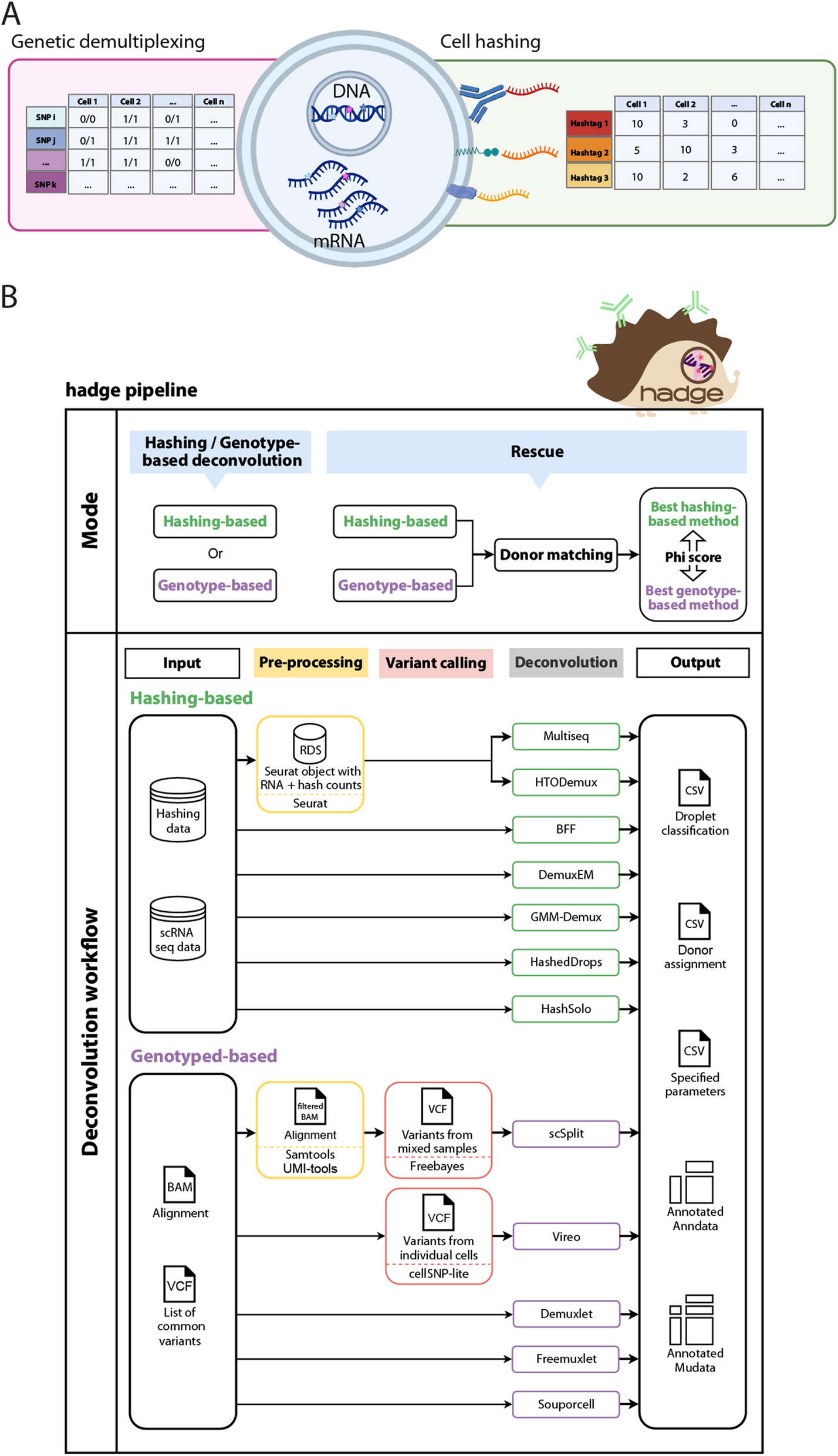
The SuperCellCyto R package is an extension of the SuperCell package adapted specifically for cytometry data. SuperCellCyto offers a practical approach to reduce the size of large cytometry data by grouping cells with similar marker expression into supercells. Figure 1A depicts the schematic overview of the generation of supercells using the SuperCellCyto R package. The process begins with performing a Principal Component Analysis (PCA) on the cytometry data to capture the main sources of variation. The number of principal components (PCs) is adjustable, with a default setting of 10, but can be increased up to the number of markers in the data. For datasets with fewer than 10 markers, the number of PCs is set to the number of markers in the data. Using the PCs, a k-nearest-neighbour (kNN) graph is constructed, with each node representing a single cell. A walktrap algorithm [36] is then applied to identify densely interconnected subgraphs or communities. This step involves performing a series of four-step random walks from each node, where a single step represents a transition from one node to another. The destination node for each step is selected randomly, and the probability of a random walk starting and ending at a given pair of nodes is used to determine their proximity. After computing these distances, nodes are iteratively merged, starting with each node in its own community, until a single community is formed, creating a dendrogram-like structure. This dendrogram is then cut at a specific level to yield the desired number of communities, referred to as supercells.

Fig. 1

The SuperCellCyto framework. A Schematic overview of the SuperCellCyto R package for generating supercells from cytometry data. B Proposed workflow for an end-to-end cytometry data analysis using supercells as the fundamental unit of analysis. The workflow begins with the generation of supercells using SuperCellCyto from cleaned and transformed cytometry data. If necessary, batch correction is then performed at the supercell level. Supercells are then clustered and annotated based on the cell type they represent. Differential expression analysis can be performed using existing tools such as Limma following aggregation of supercells at the sample and cell type level. Differential abundance analysis is performed after expanding supercells back to single cells using existing tools such as Propeller

The number of supercells generated for a given dataset is controlled by the parameter gamma, which governs the granularity of the supercells and determines at which level the dendrogram is cut. Gamma is defined as the ratio of the number of cells to the number of supercells. Choosing the appropriate gamma value involves balancing the trade-off between the data compression level and the probability of supercells encompassing diverse cell types. A larger gamma value produces fewer supercells (higher compression level), but each supercell is more likely to contain more heterogeneous cell types. Conversely, a smaller gamma value yields more supercells (lower compression level), but each supercell is less likely to contain multiple different cell types. It is important to note that each supercell may contain a different number of cells, centred around the value of gamma. We found the default value of 20 to work well for most datasets. Critically, we have implemented within SuperCellCyto the ability to adjust the number of supercells generated for a dataset without having to regenerate the kNN graph or re-running the walktrap algorithm. This feature allows users to rapidly fine tune the data compression level as required.

SuperCellCyto is designed to process each sample independently, and we have introduced the ability to process multiple samples concurrently. This is facilitated through the use of the BiocParallel R package [37] and a custom load balancing strategy. Samples are first ordered based on their cell count, and parallel workers are then tasked to process these samples in descending order, starting with the sample that contains the most number of cells. This strategy allows workers processing smaller samples to be assigned additional samples, while those handling larger samples can concentrate on their tasks without being overburdened. This approach maximises throughput and minimises idle time, thereby enhancing overall efficiency.

The SuperCellCyto R package takes as an input a transformed (using ArcSinh or Logicle [38] transformation) cytometry dataset formatted as an R data.table object [39] where each row represents an individual cell and each column denotes a marker. For each supercell and marker, SuperCellCyto calculates the marker expression of supercells by aggregating the marker expression of all cells within the supercell using either the mean or median as determined by the user. These aggregated marker expressions are outputted as an R data.table object.

Additionally, SuperCellCyto generates a cell-supercell map, also in R data.table format. This map lists each cell's supercell ID, enabling users to expand individual supercells without extra computational effort. This map is particularly useful when used in conjunction with the marker expressions of individual cells, as it allows users to access marker expressions of all the cells in a specific supercell.

Importantly, when the number of supercells is adjusted, both the supercell marker expression and the cell-supercell map are updated accordingly.

Figure 1B illustrates our proposed workflow for an end-to-end cytometry data analysis, using supercells as the fundamental unit of analysis. The first step is to pre-process the cytometry data to exclude doublets and dead cells, transform the data using either ArcSinh transformation or Logicle [38] transformation, and create supercells from the cleaned transformed single cell level cytometry data. Once supercells have been created, almost all subsequent analysis tasks can be performed at the supercell level, including batch correction (if necessary), clustering and cell type annotation, and differential expression analysis. For differential abundance analysis, we strongly recommend expanding the annotated supercells to the single cell level and calculating cell type proportions from the single cell level data. Additionally, we also recommend discarding underrepresented clusters, that is, clusters that only capture a small number of cells from each sample. For differential expression and abundance analyses, existing R packages, including those from the scRNAseq field such as Limma [40], EdgeR [41,42,43], or Propeller [22], can be used.

Supercells preserve biological heterogeneity and facilitate efficient cell type identification

We assessed whether supercells could preserve the biological diversity inherent in a cytometry dataset, and whether the clustering of supercells could expedite the process of cell type identification without compromising accuracy. We generated supercells for two publicly available cytometry datasets, Levine_32dim [7] and Samusik_all [8] (Additional file 1: Table S1) using a range of gamma values (Additional file 1: Table S2 and Additional file 1: Fig. S1). For gamma set to 20 (the default), the Samusik_all dataset was reduced from 841,644 single cells to 42,082 supercells, an approximately 20 fold reduction. Importantly, each supercell may capture a different number of cells, centred around the gamma value. The distribution of the number of cells captured in the supercells is available in the Additional file 1: Fig. S2.

Thereafter, we clustered the supercells using FlowSOM [6], a popular clustering algorithm for cytometry data, and Louvain [44], a popular clustering algorithm for analysing scRNAseq data. For both algorithms, we broadly explored their parameter space, namely the grid size and the number of metaclusters for FlowSOM, and the parameter k for Louvain (see Additional file 1: Table S3 for the list of values explored). Using the cell type annotation acquired through a manual gating process performed by the authors of the datasets as the ground truth, we evaluated the quality of the supercells by using two metrics; purity and Adjusted Rand Index (ARI). Purity quantifies the homogeneity of cell types within each supercell by measuring the proportion of the most dominant cell type within a given supercell. ARI measures the similarity between the clustering of supercells and the manually gated cell type annotation. Additionally, for ARI, we also measured the concordance between the clustering of supercells and the clustering of single cells (see Materials and Methods section for more details).

Figure 2A illustrates the distribution of supercells' purity scores across all gamma values. For both datasets, we observed very high mean purity scores across all gamma values (mean purity > 0.9, Fig. 2A), with the vast proportion of supercells attaining a purity score of 1 (Additional file 1: Table S4). We compared the purity of randomly assigned cell groups with that of supercells (Additional file 1: Fig. S3). This comparison demonstrated a vastly superior purity score achieved by SuperCellCyto, which consistently shows an average purity > 0.9. In stark contrast, random grouping typically results in a much lower purity, mostly around 0.3 and 0.4.

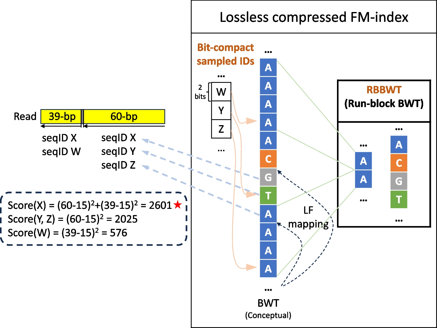
Fig. 2

SuperCellCyto preserves biological heterogeneity. A Distribution of supercell purity for Levine_32dim and Samusik_all datasets across different gamma values. Red dot denotes mean purity of the supercells. B Adjusted Rand Index (ARI) illustrating the agreement between supercell clustering and manually gated cell type annotation for Levine_32dim and Samusik_all datasets. C ARI comparison between supercell and single-cell clustering. D Identification of rare B cell subsets through clustering of supercells. Median expression of cell type markers across supercells for each cluster and B cell subsets for the Oetjen_bcell dataset. E The abundance of B cell subsets across all samples as identified by clustering supercells generated for the Oetjen_bcell dataset. Cluster 46 represents the extremely rare Plasma cells which make up only 0.002% of the cells. Only clusters annotated with B cell subsets are shown

Examining the cell types captured in each supercell, we found that the majority of supercells contained exclusively one cell type (Additional file 1: Fig. S4). While there exist instances of supercells capturing two or more cell types, they were markedly fewer. This indicates that most supercells are composed of either exclusively or predominantly a single cell type. As the gamma value increases, we observe a slight decline in both the mean purity score and the proportion of supercells obtaining a purity score of 1 (Fig. 2A and Additional file 1: Table S4) and increase in the number of supercells capturing more than one cell type (Additional file 1: Fig. S4), consistent with the fact that larger gamma values result in fewer supercells and thus higher likelihood of each supercell capturing multiple cell types. Lastly, we compared the distribution of marker expression between the supercells and single cells, and found most of them to be almost identical (Additional file 1: Fig. S5).

Upon examining the ARI computed between the supercell clustering and the cell type annotation (Fig. 2B), as well as between the clustering of supercells and single cells (Fig. 2C), we observed high scores across all datasets, clustering algorithms, and gamma values. Similar to the trend observed for purity scores, the ARI scores also exhibited a slight decline as the gamma value increased, due to each supercell encompassing a more diverse set of cell types. We noted a larger variation in ARI scores obtained for FlowSOM clustering results compared to those obtained for Louvain clustering results, potentially due to the broader range of parameter settings explored for FlowSOM (Additional file 1: Table S3).

These results collectively demonstrate that supercells can vastly improve clustering efficiency while effectively preserving the biological heterogeneity within a dataset, thereby enabling accurate clustering and identification of cell types.

Identifying rare B cells subsets by clustering supercells

Downstream analysis of cytometry data routinely involves clustering cells and subsequently manually annotating them based on their marker expression to determine the cell types they represent. While we have demonstrated that SuperCellCyto can maintain fidelity of cell types compared to cell type annotation obtained through manual gating, we next sought to verify whether we can faithfully replicate the traditional clustering and annotation process, and identify rare cell populations at the supercell level. We applied SuperCellCyto and Louvain clustering to a large flow cytometry dataset profiling more than 8 million B cells in healthy human bone marrow samples (Oetjen_bcells data [45], Additional file 1: Table S1).

Our analysis workflow consists of steps 1, 2, and 4 in Fig. 1B. First, we ran SuperCellCyto with gamma set to 20 to reduce the dataset to 415,711 supercells. We next clustered the supercells using the Louvain clustering algorithm. Based on the clustering results and known marker expression for B cells (Fig. 2D and Additional file 1: Note S1), we successfully identified all the B cell subsets present in the dataset, including the extremely rare plasma cells of which there are only 162 cells (0.002%) present at the single cell level (Fig. 2E and Additional file 1: Fig. S6A). To further validate the cell type annotation conducted at the supercell level, for each cell type, we expanded the supercells into individual cells and examined their marker expression profiles. We found them to be consistent with the manual gating scheme previously used by Oetjen et al. to identify the B cell subsets (Additional file 1: Fig. S6B and Note S1).

To demonstrate the effectiveness of SuperCellCyto, we conducted a comparison using the same dataset. From the same dataset (Oetjen_bcells data), we randomly subsampled 415,711 cells, which matches the number of supercells generated by SuperCellCyto, and then clustered them using Louvain clustering. With this subsampled data, we identified 7 out of the 10 available B cell subsets, with the loss of Activated Mature B cells, Plasma cells and Plasmablast (Additional file 1: Fig. S7). In contrast, using SuperCellCyto, we successfully identified all 10 B cell subsets, including the rare plasma cells. This result clearly demonstrates SuperCellCyto’s superior ability in preserving biological heterogeneity within the data.

Mitigating batch effects in the integration of multi-batch cytometry data at the supercell level

Cytometry experiments often generate datasets comprising millions of cells across several batches. This can introduce technical variation, known as batch effects, between samples from different batches. Batch effects stem from differences in experimental conditions and/or instruments [4]. Before proceeding to downstream analyses like clustering or differential expression or abundance analyses, it is imperative to rectify these batch effects using batch correction methods such as CytofRUV [46] or cyCombine [47] (for more details, see Materials and Methods section).

To demonstrate the feasibility of correcting batch effects at the supercell level, we applied CytofRUV and cyCombine to a large mass cytometry dataset profiling the peripheral blood of healthy controls (HC) and Chronic Lymphocytic Leukaemia patients (CLL) (Trussart_cytofruv data [46], Additional file 1: Table S1). This dataset consists of 8,589,739 cells and 12 paired samples profiled across two batches (each batch profiles one of the paired samples), yielding a total of 24 samples (Fig. 3A). Our analysis workflow consists of steps 1–3 in Fig. 1B. We applied SuperCellCyto with gamma set to 20 to reduce the data to 429,488 supercells. Importantly, as per SuperCellCyto’s default mechanism, the supercells for each sample were generated independent of other samples. This ensures that there is no mixing of cells from different samples or batches within any supercell. Following the creation of supercells, we employed CytofRUV and cyCombine for batch correction.

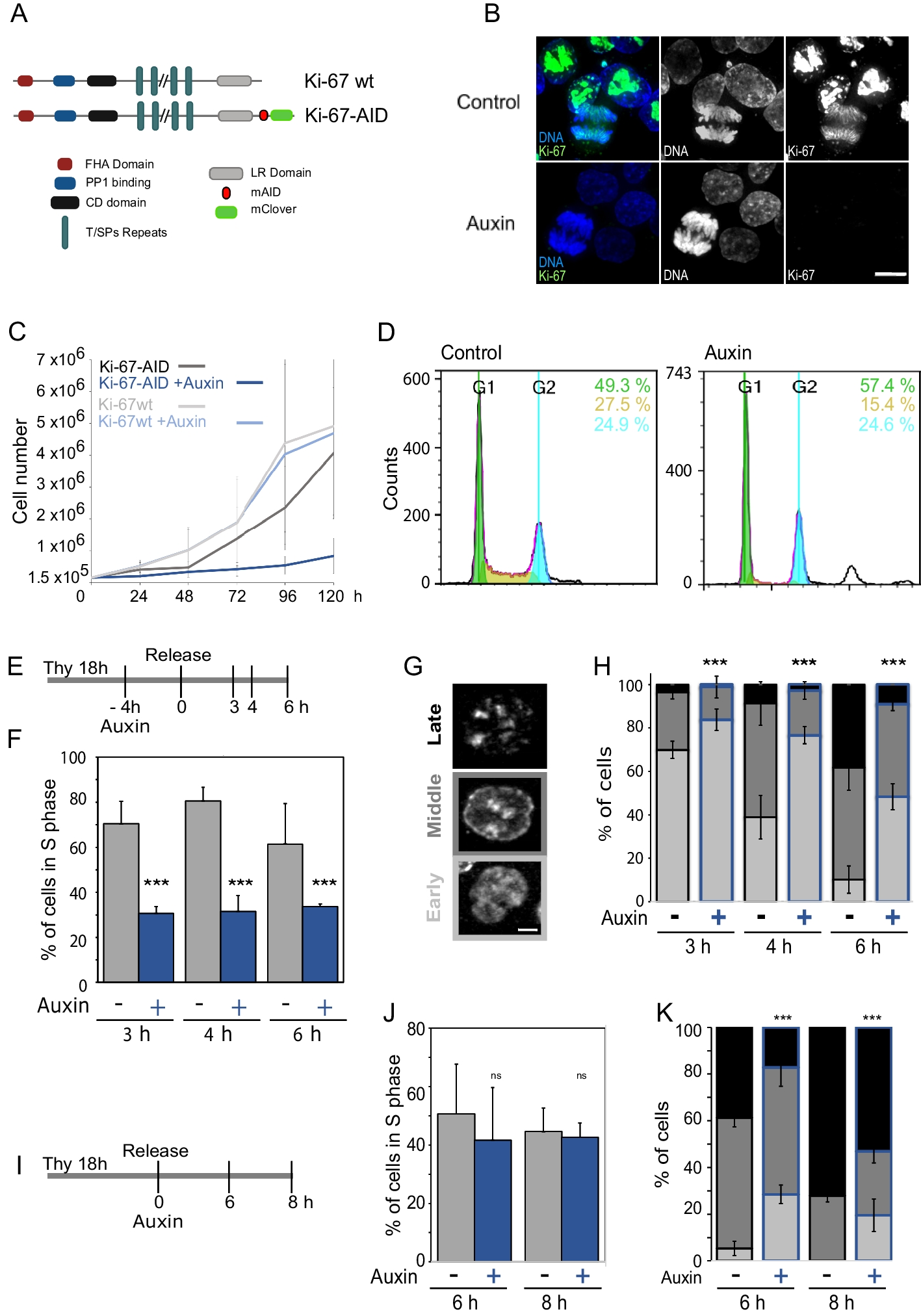
Fig. 3

Application of batch correction techniques at the supercell level. A A Multidimensional Scaling (MDS) plot showcasing the variation in uncorrected single cells, supercells, and supercells that have been batch corrected using the CytofRUV and cyCombine algorithms for the Trussart_cytofruv dataset. Each point represents a sample. B Distribution of CD14, CD45RA, and CD11c expression for uncorrected, CytofRUV-, and cyCombine-corrected supercells for Trussart_cytofRUV dataset. C Scores for metrics used to assess the preservation of biological signals of cyCombine and CytofRUV. ARI and NMI were only calculated for corrected supercells, as these metrics require a comparison with respect to the uncorrected supercells

The effectiveness of the batch correction methods was assessed through Multidimensional Scaling (MDS) analysis and comparison of the Earth Mover Distance (EMD) metric for each marker across the two batches. In addition, we also used 3 different metrics to assess the preservation of biological signals post batch correction—Adjusted Rand Index (ARI), Normalised Mutual Information (NMI), and Average Silhouette Width for labels (ASW_label). These metrics are taken from the scib package [48], renowned for benchmarking batch integration tools for scRNAseq data. Both ARI and NMI evaluate the consistency of clustering results pre- and post-batch correction while ASW_label quantifies the compactness and separation of clusters. For these metrics, the cluster labels were obtained by clustering the supercells before and after batch correction using FlowSOM [6]. All metrics were by default scaled to yield scores between 0 and 1 by the scib package, where 0 denotes poor while 1 denotes excellent performance.

Figure 3A presents the MDS plots at the sample level for uncorrected single cells, uncorrected supercells, and CytofRUV- and cyCombine-corrected supercells. In both uncorrected single cells and supercells, dimension 1 distinguishes CLL samples from HC samples, while dimension 2 separates the batches, indicating the presence of strong batch effects even at the supercell level. However, in the batch-corrected supercells, while dimension 1 continues to differentiate the CLL samples from the HC samples, dimension 2 no longer separates the samples based on their batch. This observation is further supported by the UMAP plots of uncorrected and corrected supercells, which demonstrate reduced batch-based separation following correction (Additional file 1: Fig. S8).

We compared the marker expression distribution between the two batches for uncorrected, CytofRUV-corrected, and cyCombine-corrected supercells, and found them to be more similar to one another following batch effect correction (Additional file 1: Fig. S9). This was particularly evident for CD14, CD45RA and CD11c markers (Fig. 3B).

The EMD calculated for the uncorrected and corrected supercells are shown in Additional file 1: Fig. S10. Generally, we observed a reduction in EMD score for both CytofRUV- and cyCombine-corrected supercells, indicating effective batch effect correction. Alongside the reductions in EMD scores, the visual examination of marker expression in Fig. 3B and Additional file 1: Fig. S9 indicates that the marker expression distribution post batch correction is largely preserved and not being unduly compressed (over-corrected).

Figure 3C illustrates the results for the 3 metrics employed to evaluate the preservation of biological signals following batch correction. For both cyCombine and CytofRUV corrected supercells, we observed high scores for ARI and and NMI, indicative of strong concordance in the clusterings of uncorrected and batch corrected supercells. Furthermore, there was an increase in the ASW_label score post batch correction, denoting denser and better separated clusters. Altogether, these metrics further suggest an effective preservation of biological signals post batch correction.

In summary, our analysis demonstrates that while batch effects are present at both the single cell and supercell level, they can be effectively corrected using batch effect correction methods such as CytofRUV and cyCombine following summarisation of single cells to supercells with SuperCellCyto.

Recovery of differentially expressed cell state markers across stimulated and unstimulated human peripheral blood cells

For cytometry data, a typical downstream analysis following clustering and cell type annotation is identification of cell state markers that are differentially expressed across different experimental groups or treatments. In this analysis, we assessed whether a differential expression analysis performed at the supercell level can recapitulate previously published findings obtained by performing differential expression analysis at the single cell level using the Diffcyt algorithm [11]. Specifically, we analysed a publicly available mass cytometry dataset quantifying the immune cells in stimulated and unstimulated human peripheral blood cells (BCR_XL dataset [49], Additional file 1: Table S1). Notably, this is a paired experimental design, with each of the 8 independent samples, obtained from 8 different individuals, contributing to both stimulated and unstimulated samples (16 samples in total). Importantly, this dataset was previously analysed using the Diffcyt algorithm to identify the cell state markers that were differentially expressed between the stimulated samples (BCR-XL group) and the unstimulated samples (Reference group). We refer readers to the Materials and Methods section for more information on the dataset. Our aim was to replicate these findings using a combination of SuperCellCyto and the Limma R package [40].

Our analysis workflow consists of steps 1, 2, 4, and 5 in Fig. 1B. First, we used SuperCellCyto (gamma = 20) to generate 8,641 supercells from 172,791 cells (step 1–2). We then annotated the supercells with the corresponding cell type labels (step 4) and calculated the mean expression of each cell state marker for every sample and cell type combination, akin to the pseudobulk approach commonly used in scRNAseq differential expression analysis. Next we used the Limma R package to test for expression differences between the stimulated and unstimulated samples, for each cell type separately, accounting for the paired experimental design (step 5, see Materials and Methods section for more details). Given the availability of cell type annotation, we slightly modified step 4 by annotating each supercell with the label of the most abundant cell type it encompasses, as opposed to clustering the supercells (refer to the Materials and Methods section for more details).

Our workflow successfully identified several cell state markers which show strong differential expression between the stimulated and unstimulated groups (False Discovery Rate (FDR) <  = 0.05, Fig. 4A, B and Additional file 1: Fig. S11). Our findings were consistent with those identified by Diffcyt, including elevated expression of pS6, pPlcg2, pErk, and pAkt in B cells in the stimulated group, along with reduced expression of pNFkB in the stimulated group (Fig. 4A). We also recapitulated the Diffcyt results in CD4 T cells and Natural Killer (NK) cells, with significant differences in the expression of pBtk and pNFkB in CD4 T cells between the stimulated and unstimulated groups (Fig. 4B), and distinct differences in the expression of pBtk, pSlp76, and pNFkB in NK cells between the stimulated and unstimulated groups (Additional file 1: Fig. S11).

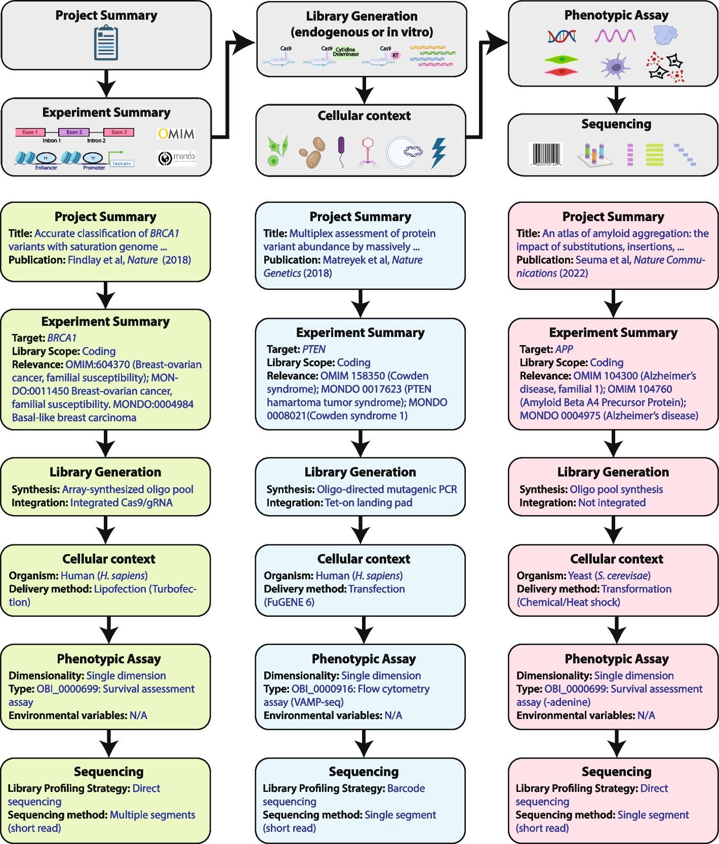
Fig. 4

Differential expression and abundance analysis using supercells. A, B Heatmaps illustrate the scaled and centred median expression of cell state markers, calculated for each sample across the supercells, for B cells and CD4 T cells in the BCR_XL dataset. Each sample (row) is annotated according to its stimulation status, either with B cell receptor / FC receptor cross-linker (BCR-XL) or unstimulated. Each marker (column) is annotated based on its statistical significance as determined by Limma at a 5% False Discovery Rate (FDR_sig). C-F Differential abundance analysis following supercell creation for the Anti_PD1 dataset. C A Multidimensional Scaling (MDS) plot showcasing the variance in samples following cyCombine correction. D Distribution of marker expression for cyCombine-corrected supercells. E The proportion of single cells for the rare monocyte subset cluster (cluster_10). F Comparison of FDR obtained by running Propeller at the single cell or supercell level. The y-axis represents the -log10 transformed FDR, with lower FDR (more significant) corresponding to higher -log10 values. The red dotted line shows an equivalent FDR of 0.1

Identification of differentially abundant rare monocyte subsets in melanoma patients

In this analysis, we investigated the capacity to conduct differential abundance analysis using supercells. We applied SuperCellCyto and Propeller [22] to a mass cytometry dataset quantifying the baseline samples (pre-treatment) of melanoma patients who subsequently either responded (R) or did not respond (NR) to an anti-PD1 immunotherapy (Anti_PD1 dataset [50], Additional file 1: Table S1). There are 20 samples in total (10 responders and 10 non-responders). The objective of this analysis was to identify a rare subset of monocytes, characterised as CD14 + , CD33 + , HLA-DRhi, ICAM-1 + , CD64 + , CD141 + , CD86 + , CD11c + , CD38 + , PD-L1 + , CD11b + , whose abundance correlates strongly with the patient's response status to anti-PD1 immunotherapy [11, 42].

Our analysis workflow consists of steps 1, 2, 3, 4, 6 in Fig. 1B. Firstly, we used SuperCellCyto (gamma = 20) to generate 4,286 supercells from 85,715 cells. We then used cyCombine to integrate the two batches together (Fig. 4C, D), and clustered the batch-corrected supercells using FlowSOM (see Materials and Methods for more details). We then identified the clusters representing the rare monocyte subset based on the median expression of the aforementioned rare monocyte subset’s signatory markers (see Additional file 1: Fig. S12A). For differential abundance analysis, we strongly recommend expanding the supercells back to single cells for more accurate cell type proportion calculation as each supercell contains different numbers of cells. Notably, expanding supercells back to single cells requires no additional computational effort. This is because SuperCellCyto readily provides a cell-to-supercell mapping which clearly identifies which supercell each cell belongs to. Once we expanded the supercells back to single cells, we retained only clusters that contained more than three cells from each sample, and performed a differential abundance test using Propeller, accounting for the batch. For comparison, we also applied Propeller directly on the supercells without expanding them back to single cells. For consistency, we only compared clusters that were retained by the filtering process.

Using the heatmap depicting the median expression of markers for each cluster (Additional file 1: Fig. S12A), we identified the rare monocyte subset as cluster 10. We found a statistically significant shift in abundance for cluster 10 between the responder (R) and non-responder (NR) groups, with responders exhibiting a higher proportion of these rare monocyte subsets (FDR <  = 0.05, Fig. 4E).

Comparing the statistical test outcomes performed at the single cell and supercell level, we found that the difference in the abundance of supercells for the rare monocyte subset (cluster 10) was also statistically significant at the FDR threshold of 0.05 (Additional file 1: Fig. S12B, Fig. 4F). While this finding is consistent with the test outcome obtained from the single cell level abundance test, broadly, we observed variations in the FDR values obtained for each cluster (Fig. 4F). Neither the single cell nor the supercell level tests consistently yielded higher or lower FDR. Hence, our recommendation is to perform differential abundance analysis at the single cell level for the most accurate results.

Efficient cell type label transfer between CITEseq and cytometry data

In this analysis, we investigated the potential for automating the annotation of cell types in cytometry data using previously annotated CITEseq data. Our workflow involves generating supercells from the cytometry data, subsetting the supercell and CITEseq data to only the common markers, and subsequently performing the label transfer process from the CITEseq data to the supercells, using either Seurat rPCA [16] or the Harmony alignment algorithm [51] combined with a kNN classifier (Harmony plus kNN). Supercells were only generated for the cytometry data, and not for the CITEseq data. For comparison, we also performed the cell type label transfer at the single cell level (single cell CITEseq to single cell cytometry). We demonstrate the effectiveness of the workflow by transferring the cell type annotation from the single cell CITEseq data generated by Triana et.al [52] to the supercells generated for the Levine_32dim mass cytometry data (see Additional file 1: Table S1).

We quantitatively assessed the effectiveness of label transfer using accuracy and weighted accuracy metrics. This involved aligning the cell type labels in the CITEseq data with those in the cytometry data. For each cell type in the cytometry data, we identified the corresponding cell type in the CITEseq data. In cases where the CITEseq data provided more granular subsets, we merged these subsets into broader categories. These broader categories were then matched with the equivalent cell type labels in the cytometry data. Specifically, for hematopoietic stem cells and progenitors, we combined the 3 subsets in the cytometry data into a group labelled CD34 + _HSCs_and_HSPCs. We then mapped the subsets in the CITEseq data which expressed the CD34 transcript or antibody to this consolidated group. Cell types lacking direct counterparts, such as Basophils in the cytometry data or Conventional Dendritic Cells in the CITEseq data, remained unchanged. Further details about this mapping process is available in the Materials and Methods section. The resulting cell type label mapping, along with the UMAP plots showing both the original and mapped cell type annotation are available in the Additional file 1: Table S5 and Additional file 1: Fig. S13.

Using the cell type label mapping described above, for each true cell type label in the cytometry data, we calculated accuracy score. This score represents the proportion of correctly labelled cells. To account for the different proportions of each cell type present in the cytometry data, we also computed a weighted accuracy score. We did this by multiplying the accuracy of each cell type by its relative proportion in the cytometry data (Additional file 1: Table S6). These weighted scores were then summed to produce an overall weight