
記住我


Test–retest sessions (Test 1, Test 2) were separated by one week between the tests (Hopkins et al. 2001). All study participants were assessed at the same time of day, using the same order of participants and subtests. In a separate familiarization test session conducted within one month prior to Test 1, all study participants were familiarized with the entire test protocol; questionnaires, body composition measurements, warm-up, countermovement jump testing, assessments of maximal muscle strength and RTD for the knee extensors and flexors, and measurements of 20-m sprint capacity with and without dribbles with handball (see Fig. 1). All instructions and steps of data collection were managed by the same assessor at both tests. Standardized oral instructions were provided to all players before initiation of each test.
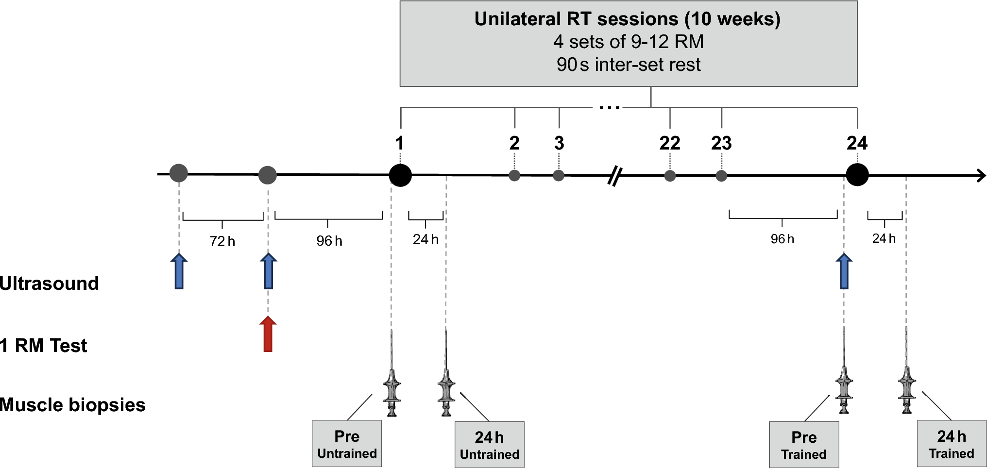
Fig. 1
Estimated timeline for the test protocol. Study participants started by filling in an online questionnaires on their mobile device. Bodycomposition was measured followed by standardized warm-up, countermovement jump test, maximal voluntary contraction strength test of the knee extensors and flexors and lastly 20-m sprint with and without ball
SubjectsSixty female youth elite team handball players from the Danish U17 and U19 league agreed to participate in the study. Twenty players completed all three test sessions (Table 1). Study participants received written and oral information about the experimental procedures prior to giving their written informed consent. Parental or guardian signed consent was obtained from subjects < 18 years. The study was registered at the Regional Committees on Health Research Ethics for Southern Denmark (20,212,000–114). Subject characteristics are listed in Table 1.
Table 1 Participant characteristicsBody compositionBioimpedance (InBody 270, InBody Co., LTD, Seoul, South Korea) measurements were performed to assess body mass (BM), skeletal muscle mass (SMM) and fat percentage (FAT%). Body height was measured twice (Leicester Height Measure Mk II, Child Growth Foundation, Newcastle, England) and an average was calculated. Athletes were not subjected to any restrictions on energy-intake before the measurements.
Warm-up procedureAll study participants completed a standardized ~ 10-min warm-up program. The warm-up program consisted of running, strength exercises and ball throws. Half-court dash runs; 4 × low-to-high intensity runs, 2 × sidesteps, 1 × backwards run and 2 × skip running. Body weight strength exercises were: 10 × squat, 10 × single-leg Romanian deadlift (5/5), 10 × sit-ups, 10 back extensions, 10 × push-ups, 20 × single-leg medio-lateral leg swings (10/10), 20 × single-leg anterior–posterior leg swings (10/10), 20 × forward and backward arm swings (10/10) for each arm, followed by 8 × single-leg jumps (4/4), and 8 × random change of direction movements. Lastly, participants performed 20 × ball throws (10 × medium velocity, 10 × high velocity).
CMJ performance (SSC muscle power)Stretch–shortening cycle (SSC) muscle performance was assessed in a bilateral countermovement jump test performed on an instrumented force plate (AccuPower, AMTI, Watertown, USA) (Caserotti et al. 2001; Bojsen-Møller et al. 2005). Two initial submaximal warm-up jumps were performed followed by five maximal single effort jumps, each interspaced by 30-s recovery. Subjects were instructed to execute the jump in a continuous movement, while focusing on jumping as high and forcefully as possible with their hands positioned on the hips (Caserotti et al. 2001; Thorlund et al. 2008; Jakobsen et al. 2012). Vertical ground reaction force (Fz) signals were A/D converted at 1000 Hz using custom build software script (MATLAB, MathWorks, Natick, USA). During later off-line analysis, the Fz signals were analyzed also using custom build software script (MATLAB, MathWorks, Natick, USA), where the jump with the highest jump height was chosen for further statistical analysis. All CMJ take-offs were divided into an eccentric (downward) phase (Ep) and a concentric (upward) phase (Cp), the former defined as the time interval with downward body center of mass (BCM) movement to its deepest position (V = 0) and the latter defined as the upward BCM movement from its deepest position to toe-off (Caserotti et al. 2001; Thorlund et al. 2008; Jakobsen et al. 2012). Ep was further divided into an eccentric acceleration phase (Ep-acc), the interval from onset of downwards movement to the instant of maximal negative (downwards) BCM velocity (Vpeak [Ep]), and an eccentric deceleration phase Ep-dec, defined as the interval from Vpeak (Ep) to BMC deepest position (V = 0) (Caserotti et al. 2001; Thorlund et al. 2008; Jakobsen et al. 2012). Vertical jump height was calculated as \(}}_}}^/2}\) where Vto denotes the take-off velocity of BCM calculated from time integration of the net upward ground reaction force (Fz) during the concentric take-off phase \((}_}}} \, = \,\int }_}} /}} \right) - }} \right] \cdot }t)}\), BM = body mass (kg), gravitational acceleration (g = 9.81 m/s2) (Bojsen-Møller et al. 2005; Holsgaard Larsen et al. 2007; Jakobsen et al. 2012). Besides maximal vertical jump height, jumps were analyzed for jump height relative to ground level (JHGL), calculated as JH + (BCMdisp [Cp] – BCMdisp [Ep]), peak and mean take-off power, work exerted on BCM, rate of force development (RFD) calculated as the average tangential slope at 0–100 ms relative to the start of the Ep-dec, duration of the concentric take-off phase (Cp; BCM moving from deepest position to toe-off), BCM displacement (BCMdisp) in the Ep and Cp, and lower limb stiffness (LLS) calculated as LLS = ΔvGRF/ΔBCMdisp (Ep), where ΔvGRF is change (Δ) in vertical (v) ground reaction force (GRF) (Jordan et al. 2023).
Isometric knee extensor and flexor strengthMVIC peak torque was measured for the knee extensors and flexors of the dominant leg (take-off leg in jump-shooting), along with the assessment of RTD and impulse using a portable isometric dynamometer (Dynamometer, Science to Practice (S2P), Ljubljana Slovenia). Anatomical knee joint angle was (mean ± SD) 50.2 ± 3.2° and 46.3 ± 4.1° for the knee extensor and flexor MVIC tests (0° = full knee extension), respectively, as measured with goniometry (Baseline®, HiRes® 360° 30-cm, Fabrication Enterprises Inc., White Plains, NY, USA). These configurations were applied due to mechanical constraints of the dynamometer and the objective of identical anatomical knee joint angle for knee extensors and flexors, respectively, to evaluate H/Q-ratios (Maffiuletti et al. 2007). Seat position and external lever arm lengths (distance from knee joint rotation center to point of ankle cuff attachment) were individually adjusted for each study participant to 2-cm above the lateral malleolus (Aagaard et al. 2002). Subjects were firmly strapped to the chair seat and backrest (10° reclined) at the hip and distal thigh. Individual seat and ankle cuff positions were the same at Test 1 and Test 2. All recorded muscle torques were corrected for the effect of gravity on the lower limb (Aagaard et al. 1995).
Subjects performed two submaximal warm-up contractions followed by five contractions at maximal voluntary effort for the knee extensors and knee flexors, respectively, with 1-min recovery between trials. The assessor provided strong verbal encouragement and study participants simultaneously received visual online feedback of their exerted torque (Aagaard et al. 2002; Maffiuletti et al. 2007; Fristrup et al. 2020). All participants were carefully instructed to contract as fast and forcefully as possible and maintain the contraction for 4–5 s or until otherwise instructed by the assessor (Fristrup et al. 2020). Knee joint torque was measured with a strain gauge-based force sensor and calculated into torque (model Z6FC3-200 kg, Hottinger-Baldwin Messtechnik GmbH, Darmstadt, Germany). The torque signal was sampled at 1000 Hz using the built-in dynamometer software (ARS dynamometry, S2P ltd., Ljubljana, Slovenia). Raw torque signals were then exported for subsequent processing and data analysis using custom build software script (MATLAB, MathWorks, Natick, USA). All recorded torque signals were low pass filtered using a digital fourth-order, zero-lag Butterworth filter with a cutoff frequency of 15 Hz (Aagaard et al. 2002; Bojsen-Møller et al. 2005; Fristrup et al. 2020). MVIC peak torque was defined as the highest peak torque value among the trials, while onset of torque was defined as 1% of MVIC. Trials with pre-contracting torque exceeding 1% of MVIC peak torque were discharged. For the statistical analysis of knee extensor and flexor MVIC, along with the calculation of hamstring-to-quadriceps strength ratios (H/Q-ratio), the trial with highest MVIC peak torque was chosen for analysis.
Impulse is represented by the area under the torque–time curve, calculated as ∫Torque dt with t being time (Aagaard et al. 2002). Impulse reflects the angular speed of the lower limb if it had been allowed to move freely, thus it might be the most functional measure of rapid muscle torque production in an isometric contraction (Maffiuletti et al. 2016). For the evaluation of RTD and impulse, the trial with highest impulse at 0–200 ms was selected for further statistical analysis since this measure represents the integrated time-history of contraction throughout entire time interval of 0–200 ms. Rate of torque development and impulse were calculated as the slope (Δtorque/Δtime) and the area (∫Torque dt), respectively, of the torque–time curve in the initial (early) time intervals (0–30 ms and 0–50 ms) and later time intervals (0–100 ms and 0–200 ms) relative to onset of contraction (Aagaard et al. 2002; Andersen and Aagaard 2006; Jordan et al. 2015; Maffiuletti et al. 2016; Palmer et al. 2021).
Sprint performanceSprint performance was evaluated in a 20-m maximal sprint test with target finish line at 25-m and visual markings at 5, 10, 15, 20, and 25-m (Fig. 2a). Split times were collected at 5, 10 and 20-m at hip height (75-cm), using dual-beam photocells (8 MHz Wireless Training Timer (WITTY-gates), Microgate, Bolzano, Italy). Participants started from a standing position with the front foot placed at the starting line and with the start sensor placed 20-cm behind the starting line, resulting in the beam of the start sensor being interrupted by the malleolus of the front foot. When the front foot was lifted from the start position, time would begin. Study participants performed two submaximal runs at ~ 60% and ~ 80% of maximal intensity, respectively, before completing five maximal 20-m sprints, interspaced by 1-min recovery. Subjects initiated their own start (no external cueing) after the 1-min recovery within a 15-s time window. The fastest 20-m sprint time was selected for further statistical analysis.
Fig. 2
A schematic overview of the 20-m sprint test without dribbling a handball (a) and with dribbling a handball (b). Bold black lines mark start line, finish line and target finish line (25 m). Symbols of green circles with cross symbols shows photocells and yellow cones are visual markings at 15 and 25-m. In b, the 20-m sprint test with handball dribbles is illustrated
Subsequently, the participants engaged in five maximal 20-m sprints, while the subjects concurrently dribbled a handball, again interspaced by 1-min recovery. Standard rules of team handball were applicable, and resin was utilized. The starting position and split distances were the same as without ball. In the starting position, the ball was placed on top of a 35-cm high cone, with the participants instructed to touch the ball. Subjects performed two steps before the first dribble, releasing the ball before reaching the 5-m mark, and unrestricted dribbles were allowed between the 5- and 20-m marks (Fig. 2b). Dribbles were counted to ensure an identical number of dribbles at both test sessions. In addition, subjects were instructed to perform a single dribble between the 20- and 25-m mark, to ensure sustained ball control while crossing the 20-m finishing line.
Statistical analysisData were examined for normal distribution by visual inspection of QQ plots. Paired students t-testing was applied to test differences of means between Test 1 and Test 2. Significance level was set at p ≤ 0.05 (two-tailed testing). Delta values (Test 2 – Test 1) exceeding ± 2.5 standard deviations were defined as outliers (Nielsen et al. 2017) and disregarded from the analysis. Test–retest reliability were calculated by Intraclass Correlation Coefficients (ICC), two-way random effect model (ICC2,1). ICC values ≥ 0.75 were considered excellent, 0.60–0.74 good, 0.40–0.59 moderate and < 0.39 poor (Fleiss 1986; Cohen 1988). Within-subject coefficient of variation (CVw-s) was calculated as standard deviation (SD) relative to the mean (\(\overline\)) as previously described (Holsgaard Larsen et al. 2007):
$$CV_} = \frac}}} \cdot 100$$
where
$$SD = \sqrt } \right)}}} }\,d = } 2 - } \, 1$$
$$\overline = \frac_}} + \overline_}} }}$$
CVw-s ≤ 15% were considered acceptable (Dos’Santos et al. 2019; Palmer et al. 2020). Critical difference (%) was calculated with a 90% probability in this study for each examined variable, to estimate a significant change between two consecutive measurements (i.e., pre and post) for an individual of the study population or with a similar physiological profile. Critical difference (CD) was calculated as \(}= Z \cdot \sqrt \cdot }}_\), in which Z denotes the percentage points of the Gaussian distribution for a two-tailed probability of 90% (Z = 1.65) (Hayes et al. 2014; Holsgaard Larsen et al. 2007).
留言 (0)