In the first half of the study, we validated the new method by simulation, and in the second half, using this method, we conducted a clinical study on actual real-world data. As the subject of the latter half of the study, we estimated the effect of the specific health guidance provided in Japan, on the prevention of diabetes onset and medical expenditures. This subject was chosen because the effect of lifestyle guidance in preventing the onset of diabetes is almost self-evident (Muramoto et al. 2014), making it difficult to conduct an RCT from an ethical perspective. Therefore, real-world evidence is required to estimate this effect. This observational cohort study used administrative claims data and was approved by the Ethics Committee of Nara Medical University (approval no. 1123–7, October 8th, 2015).
2.1 Outline for a new method: exact-matching algorithm using administrative health claims database equivalence factors
This novel method is based on a very simple idea: according to the TTE concept, an ideal study in terms of comparability (= Target Trial) should have all covariates, except exposure, matched in both groups. However, the key to this simple approach is to match each of the covariates, not just the representative values of the covariates, as in an RCT or the PS in an observational study. This differs from traditional statistical methods, in that all measurable factors, including interactions of any order, are controlled. It is also characterized by the fact that the differences in the covariates are always zero and not distributed, regardless of the stratification of the analysis. Administrative health claims database equivalence factors (AHCDEFs) are collected from administrative claims databases and can confound exposure and outcome. The weighting factor for the group with a smaller number of people therein without exposure, and the group with exposure, among those with perfectly matched AHCDEFs, was set to 1, so that the sum of the weighting factors for the group without exposure and the group with exposure, was equal. For example, consider a simple case in which the AHCDEFs are age, gender, and systolic and diastolic blood pressure: consider a 42-year-old male with a systolic/diastolic blood pressure of 130/80 mmHg. The control for that case is a 42-year-old male with a blood pressure of 130/80 mmHg. Here, all four items are matched in the case and the subject; along with the four items, the 11 interaction terms of any combination of the four items are also controlled. The difference in this approach, compared to the conventional method that assumes agreement of representative values in the population, is that we are able to control for interaction terms of any order in the model.
2.2 Simulation procedure
The trials were conducted 500 times, independently (\(}=\mathrm, \cdots , 500\)) considering the misclassification and chance errors of all variables and competing events of outcome. The simulation process followed a sufficient causal model (Liang et al. 2014). Thus, it is only when there are equal or more than one sufficient causes that an event occurs. For each patient (\(}=1, 2, \cdots , 50 000\)), we constructed a confounding model of exposure (\(_\)) and outcome (\(}}_\)) of interest. That is, there was no difference in the true proportions of outcome occurrence between the groups with and without exposure, and the true odds ratio of outcome occurrence for the group exposed to the group without exposure was 1. \(_\) is the low-to-moderate correlated variable. \(_\) is observable, \(_, \cdots , _\) contain both observable and unobservable variables. Any of the latter 99 variables causes Y. to estimate the effect of \(_\) on \(}}_\), when only some component causes are observable and known and there may be some noncausal factors being mistaken as causal factors. Thus, we have
$$P\left(}}_=1|_,}}_ \right)=\frac__+\sum_^__}}_\right)}}\left(__+\sum_^__}}_\right)}$$
If \(}}_\) is an observable and known risk factor, \(}}_=1\), otherwise \(}}_=0\) (\(}=2, \cdots , 100\)). For some \(}, }}_=1\) and \(}}_\) is a sufficient cause of Y. \(_\) is the estimated effect of \(_\) on \(}}_\) if \(}}_=1\). In summary, \(_\) is a factor that is observed and is not a sufficient cause of Y. Among the remaining 99 \(_\), there is at least one that is a sufficient cause of Y with \(}}_\)= 1. When \(}}_\)= 0, \(_\) is either unobservable or observable (as not a risk factor).
2.3 Details of the simulation
To set low-to-moderate correlated variables \(_,_, \cdots , _\), independent random sampling of \(}}_\) and \(}}_\) was performed from uniform [0,1) distributions. All \(}}_\) are 500 × 100 × 50,000 independent samples, and all \(}}_\) are 500 × 50,000 independent samples. Independent random sampling of \(}}_\) was performed from uniform [0.3,0.6) distributions. All \(}}_\) are 500 × 100 independent samples. For \(j\)=\(1, \cdots , 9,\) \(}}_\) takes on a random value, drawn from a uniform [0.5, 0.9) distribution. All \(}}_\) are 500 × 9 × 100 independent samples. \(_\) is an unknown value based on an exact threshold value, with no misclassifications. \(_\)=1, if a linear combination of variables \(}}_}}_+}}_\left(1-}}_\right)\)>\(}}_\). \(_\)=0, if a linear combination of variables \(}}_}}_+}}_\left(1-}}_\right)\le }}_\). \(_\) is the known value, based on the expected threshold value of a uniform [0.5, 0.9) distribution, that is, 0.7 with some misclassifications. \(_\)= 1 if the linear combination of variables \(}}_}}_+}}_\left(1-}}_\right)\)>\(0.7\). \(_\)= 0 if a linear combination of the variables \(}}_}}_+}}_\left(1-}}_\right)\le 0.7\).
\(_\) takes a random value, drawn from the Bernoulli distribution, with a probability of success of 0.05. All \(_\) are 500 × 9 × 50,000 independent samples, which indicate whether a linear combination of variables \(}}_}}_+}}_\left(1-}}_\right)\) is a component of the \(j\) th possible sufficient cause. Let \(_=1\), when all components for the jth possible sufficient cause are active in the \(n\) th observation of \(t\) th trial, that is \(\sum_^__ =\sum_^_\). If \(\exists },j\) \(\sum_^__ <2,\) all variables are redetermined through the same \(j\) th random process in the \(}\) th trial. \(_\) takes on a random value, drawn from the Bernoulli distribution, with a probability of success of 0.5. All \(_\) are 500 × 9 × 50,000 independent samples, which show whether each of the nine possible sufficient causes is a real sufficient cause. If there is no real sufficient cause, that is, \(\exists \mathrm\sum_^_\)= 0, then all variables are redetermined through the same random process in the \(}\) th trial.
\(_\), and \(_\) take a random value, drawn from the Bernoulli distribution, with a probability of success of 0.001. All \(_\) are 500 × 50,000 independent samples, which indicate competing events for the outcome. All \(_\) are 500 × 50,000 independent samples, indicating a small error in the outcome.\(}}_=1\) where \(_\)= 1, and where \(\sum_^__\ge 1\) and \(_=0\); otherwise \(}}_=0\). \(}}_\) is a random value, drawn from the Bernoulli distribution, with a probability of success of 0.1 + \(\sum_^__\), which indicates whether \(_\) is an observable and known risk factor for the outcome.
2.4 Adjustment by new methods
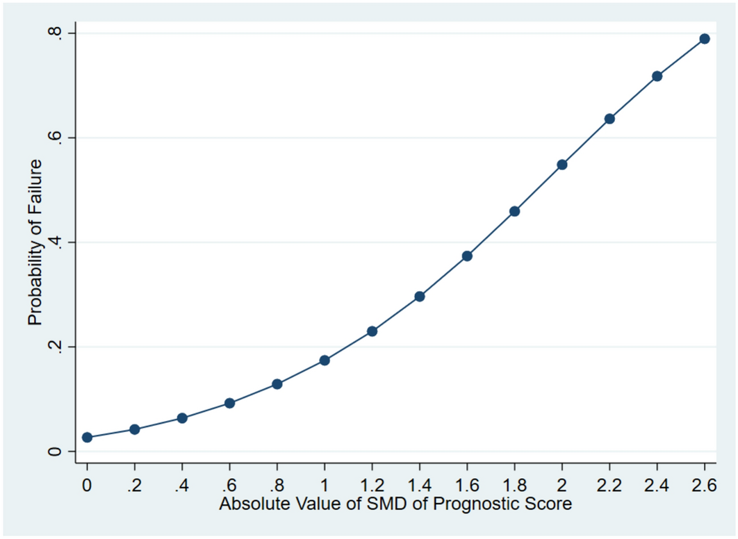
In the above model, there was no difference in the true proportion of outcome occurrence between the groups with and without exposure. However, the bias in the model resulted in an apparent difference in the proportion of outcomes. To visualize the extent to which the bias was adjusted by our proposed method, we simulated \(P\left(}}_=1|_=1\right)-P\left(}}_=1|_=0 \right)\) with and without adjustment.
2.5 Comparison with conventional methods
Two conventional methods, multivariate analysis and PS, were compared using this method (Seeger et al. 2005; Schneeweiss et al. 2009). In the model, the true odds ratio of outcome occurrence for the group exposed to the group without exposure was 1. Specifically, the odds ratios \(_\) of the three methods were compared. Type I error is the probability of erroneously determining that there is a difference when, in fact, there is no difference. Similarly, the probabilities of Type-I errors for the three methods were determined. In the PS analysis, PSs themselves were used as covariates in the regression model, because the variance in both groups was not very different (Rubin 1979).
2.6 Application to real-world data: data source
In the demonstration of the methodology, the study cohort comprised anonymized data of individuals in the Kokuho database (KDB) of Nara prefecture in Japan. This data provided information on personal identifiers, date, age group, sex, description of the procedures performed, World Health Organization International Classification of Diseases (ICD-10) diagnosis codes, medical care received, medical examinations conducted without the results, prescribed drugs, and specific health check-ups, including results from 2013 to 2021.
2.7 Study population
We included data on individuals who underwent specific health check-ups between April 2014 and March 2021. Those who were not followed up in the past year and those who were prescribed diabetic medications in the past year were excluded.
2.8 Definition of diabetes
A validated algorithm was used to define diabetes based on claims data from Japan. This algorithm (74.6% sensitivity and 88.4% positive predictive value), for detecting people with diabetes, had three elements: the diagnosis-related codes for diabetes without the “suspected” flag, the medication codes for diabetes, and these two codes on the same record (Nishioka et al. 2022). This algorithm cannot detect people with diabetes who have not consulted a doctor and those on diet and exercise therapy only, but it can identify most of them on medication.
2.9 Effect of the specific health guidance
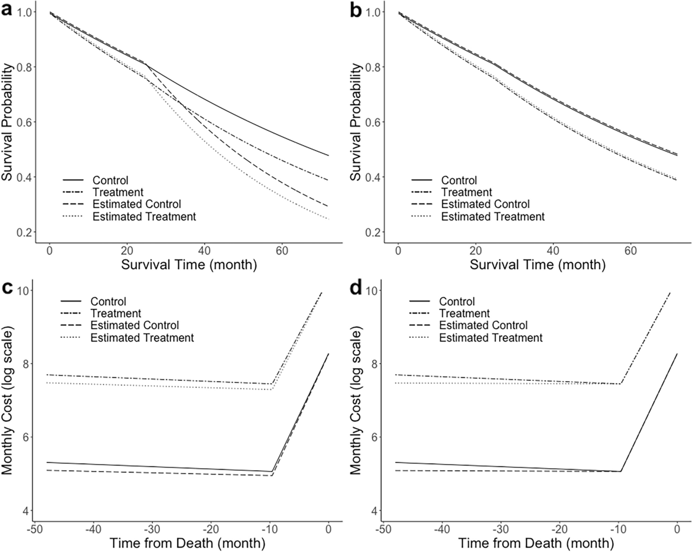
Among those who received the specified health check-up during the six-month period, those who received health guidance were identified and designated as the health guidance group. Those whose age, sex, body mass index (BMI), abdominal circumference, medical expenses in the past year, the number of days of outpatient visits in the past year, and the number of days of hospitalization in the past year matched those of the health guidance group were identified and designated as the control group. In the health guidance and control groups, odds ratios for new onset diabetes were calculated. Generalized estimating equations were used in the analysis, and a binomial distribution was assumed for the outcome of diabetes. The link function was assumed to be a logit. In an additional analysis, average medical expenditures per person per month, for both groups, were observed over time. All statistical tests were two-tailed, and P-values < 0.05 were considered statistically significant. All statistical analyses were performed using the Microsoft SQL Server 2016 Standard (Microsoft Corp., Redmond, WA, USA) and IBM SPSS Statistics for Windows, version 27.0 (IBM, Armonk, NY, USA).


留言 (0)