1 INTRODUCTION

Since its emergence, the field of non-invasive functional magnetic resonance imaging (fMRI) has been dominated by studies using blood-oxygenation level dependent (BOLD) imaging. BOLD fMRI is a powerful technique for functional paradigms, in which stimuli can be presented multiple times during an experiment. Arterial spin labeling (ASL) is an alternative fMRI method that is better suited to investigate single events, slow changes, or tonic processes such as the administration of a pharmacological agent, the induction of stress, mood states, or acute pain (Wang et al., 2003). As such, ASL is especially suited to investigate acute pain experimentally (Loggia et al., 2019).

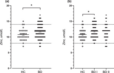
Pain processing in patients diagnosed with borderline personality disorder (BPD) seems to be altered compared to healthy controls. Overall, pain sensitivity seems to be reduced in those patients (for a review see (Schmahl & Baumgärtner, 2015)). At the same time a substantial number of BPD patients show non-suicidal self-injurious behavior (NSSI) (Zanarini et al., 2008). Although there are several motives, one of the major reasons for NSSI is relief from aversive inner tension (Kleindienst et al., 2008). Most frequently used NSSI methods comprise tissue injury (Andover et al., 2010; Kleindienst et al., 2008; Turner et al., 2015). However, there is evidence that nociceptive stimulation rather than tissue injury contributes significantly to the reduction of aversive tension (Willis et al., 2017). Using BOLD fMRI to investigate pain processing in BPD may threaten the ecological validity of the experiment, as stimuli must be presented multiple times. As ASL can be used with low-frequency designs, it constitutes an interesting alternative method.

To date, experimental pain studies using ASL in healthy controls utilized hot or cold temperature stimuli (Clewett et al., 2013; Frölich et al., 2012; Maleki et al., 2013; Owen et al., 2008; Zeidan et al., 2011; Zeidan et al., 2014), pressure (Frölich et al., 2012), deep muscular pain (Owen et al., 2010), or chemical noxious stimulation with capsaicin (Segerdahl et al., 2015). The most frequently applied NSSI method, however, is cutting (Kleindienst et al., 2008; Turner et al., 2015). To our knowledge, no ASL study so far has investigated pain responses to sharp mechanical pain. In order to address this gap in the literature, we employed a recently developed human surrogate model of incision pain (Shabes et al., 2016) to investigate the brain's response to sharp mechanical pain. The goal of the present study was to evaluate ASL as an application for examining neuronal pain processing in BPD patients. Specifically, we examined if ASL has the sensitivity to detect changes in perfusion within core areas of the nociceptive network applying a single block of sharp mechanical painful stimuli in healthy controls.

Three meta-analyses of neuroimaging studies (Apkarian et al., 2005; Duerden & Albanese, 2013; Jensen et al., 2016) identified regions with high probability to be involved in pain processing in healthy subjects across pain types. According to their results, we hypothesized to find changes in perfusion due to painful stimulation in S1, S2, insula, ACC, PFC, thalamus, and cerebellum. Although the encoding of pain intensity is most probably the result of the dynamic interplay between many different brain regions of the nociceptive network (Wager et al., 2013), the posterior insula has been proposed to be a key node (e.g., Frot et al., 2007; Isnard et al., 2011; Segerdahl et al., 2015). It is involved in sensory processing of the pain experience (Bastuji et al., 2016; Frot et al., 2014), and a number of studies have found it to be associated with pain intensity coding (Bornhövd et al., 2002; Coghill et al., 1999; Frot et al., 2007; Iannetti et al., 2005). Moreover, it is the only cortical region where pain could be elicited by electrical stimulation (Mazzola et al., 2009). Using ASL, two studies found positive correlations between regional changes in blood flow within the insula and pain intensity ratings (Owen et al., 2010; Segerdahl et al., 2015). Since the combination of ASL with mechanical stimulation is novel, we wanted to be certain to focus on the area that would most likely show a response. Hence, as a proof of concept, we hypothesized that we could detect a positive correlation between perfusion in the posterior insula and pain intensity ratings using ASL and a single block of painful mechanical stimulation.

2 METHODS AND MATERIAL 2.1 Subjects

We analyzed datasets from 19 female healthy subjects (age range: 21–39, mean: 26.4 ± 6.2 standard deviation) that were included after screening to exclude any history of neurological and psychiatric conditions, chronic pain states, regular use of medication, and MRI contraindications. Informed consent was obtained, and experimental procedures were approved by the local ethics committee (2015-600N-MA) in accordance with the Declaration of Helsinki. We initially recruited 26 healthy subjects for this study, of which seven were excluded from the final analysis. Four subjects did not complete full screening, 1 dataset had to be dismissed due to technical problems during the MRI measurement, 1 due to strong subject movement, and another due to failure of the normalization procedure during preprocessing. All participants were recruited by advertisement in newspapers or flyers, distributed at the Medical Faculty Mannheim of the University of Heidelberg.

2.2 ASL technique

In ASL, arterial blood water is used as an endogenous tracer. This is accomplished by magnetically labeling spins in arterial blood water. There are different methods to achieve labeling (pulsed ASL, continuous ASL and pseudo-continuous ASL), and each labeling scheme has its own strengths and weaknesses (see e.g., Borogovac & Asllani, 2012; Günther, 2014; for a comprehensive discussion and summary). It is important to note, however, that ASL has a lower SNR compared to BOLD fMRI. Specifically, only approximately 1% of the total signal is caused by blood delivered to the tissue. This disadvantage may be counterbalanced by decreased inter-subject variability in ASL compared to BOLD fMRI (Liu & Brown, 2007). However, ASL techniques have constantly been improved over the years with respect to SNR. For an overview of recent advancements in ASL, please see Hernandez-Garcia et al., 2019. According to the recommendations of the ISMRM Perfusion Study Group and the European Consortium for ASL in Dementia (Alsop et al., 2014), we employed a sequence with the pseudo-continuous labeling technique, in which arterial blood water is magnetically labeled in a plane beneath the brain and perpendicular to the main feeding arteries in the neck. The labeled blood is given time to diffuse into the capillary system of the brain before the MR image is read out. In order to obtain a perfusion-weighted image, a second image is needed in which no labeling is applied. Because the magnetic label reduces the signal in the image, the labeled image needs to be subtracted from the non-labeled image in order to obtain a perfusion-weighted image. As a consequence, any slow drifts present in the signal are removed and data points in a time-series of images can be meaningfully compared to each other. Moreover, perfusion values can be quantified in absolute units of ml/g/min.

2.3 Mechanical pain stimulation device

Shabes et al. introduced a stimulation device as a model of sharp mechanical pain. The device consists of a blunt blade of 4 mm length and 100 μm width that is attached to a plastic mounting and a steel tube (see Figure 1; see also Shabes et al., 2016). A moving weight (4096 mN) inside the tube ensures that the blade can be applied with constant force. In their study, Shabes et al. showed that the pain experience during 7 s of stimulation with a blunt blade is comparable to the pain experience after an incision with respect to sensory and affective properties (Shabes et al., 2016). The stimulator was developed according to the findings of Greenspan and McGillis (1991) and Slugg et al. (2000, 2004) who tested pin-prick stimuli of different force and tip dimensions in psychophysical experiments in humans and single fiber recordings in monkeys (Greenspan & McGillis, 1991). These stimuli primarily activated Aδ-nociceptors together with C-fiber nociceptors. Since the stimulator touches the skin, Aβ-fibers are likely to be coactivated as well, but with much less specificity and brief transient firing (Perl, 1968).

Schematic representation of the paradigm. Mechanical pain was applied with a blunt blade to the left forearm within an area of approximately 7 cm2 (shaded area in light red) for 96 s. Pain ratings were acquired 5 min after pain offset

2.4 Duration of stimulation block

ASL is well suited for low-frequency paradigms (Aguirre et al., 2002; Wang et al., 2003), in which few but relatively long experimental events are under investigation, such as the effect of pharmacological agents or psychological and physiological states. An example for the latter category is acute pain. Most experimental pain studies using ASL applied stimulation that added up to at least 2 min of total stimulation time (2 min: Maleki et al., 2013; 3 min: Zeidan et al., 2011; 5 min: Frölich et al., 2012; Owen et al., 2008). Others have employed paradigms with more than 15 min of painful stimulation (Owen et al., 2010; Segerdahl et al., 2015). Aguirre et al. have shown that at task frequencies below 0.009 Hz perfusion MRI starts to outperform BOLD fMRI in terms of relative sensitivity (Aguirre et al., 2002). That corresponds to a blocked design wherein a 60 s task alternates with 60 s of baseline measurement. Wang et al. demonstrated that the functional signal-to-noise-ratio (SNR) on group maps, based on perfusion measurements, are relatively constant between designs with blocks of 30, 60, 150, and 300 s of finger tapping, respectively (Wang et al., 2003). In order to increase ecological validity, we applied only one block of stimulation with no repetition. We tested 64 versus 96 s of painful stimulation in a pre-pilot study (unpublished data) and decided for the longer stimulation duration of 96 s for the present study, as it confers higher sensitivity to detect pain-related changes.

2.5 Assessment of mechanical pain thresholds and pain sensitivity 2.5.1 Pain thresholds

Mechanical pain thresholds were quantified using seven different forces of pin-prick stimuli: 8, 16, 32, 64, 128, 256, and 512 mN. These stimuli are part of the quantitative sensory testing protocol by the German Research Network on Neuropathic Pain (Rolke et al., 2006). Pin-pricks were applied at a rate of 2 s “on”/2 s “off” in ascending order until participants reported a sharp sensation and in descending order until participants reported a blunt sensation. This procedure was repeated five times for each subject, and the mean of the five thresholds was used as a final measure of the average mechanical pain threshold.

2.5.2 Pain intensity and unpleasantness

Ratings of acute blade-induced pain were acquired after the scanning sessions, to prevent confounding changes in perfusion rates due to rating and motor response activity. Participants had to verbally indicate on a numerical rating scale ranging from 0 to 100 how intensely (0 = “no pain at all”, 100 = “most intense pain imaginable”) and aversively (0 = “no pain at all”, 100 = “most aversive pain imaginable”) they perceived the stimulation. That is, we acquired a single pain intensity rating and a single pain unpleasantness rating for the complete pain stimulation period (96 s) 5 min after stimulation offset.

2.6 Experimental design

The MRI measurement started with a baseline scanning period of 120 s to ensure that the subjects had the opportunity to get used to the scanner and measurement noise and the ASL signal could stabilize. The baseline measurement was followed by 12 consecutive pain stimuli that were applied to the left forearm within an area of approximately 7 cm2. The blade stimulator was hand-held and slightly moved from one application to the next in order not to stimulate the same spot repeatedly. The application did not follow a specific pattern. The blade orientation varied randomly. Each single stimulus lasted 6 s followed by 2 s stimulation offset, resulting in one stimulation block lasting 96 s in total. In order to ensure that the stimulus timings were exact, we programmed a visual display that was projected onto a monitor behind the scanner. The monitor was only visible to the experimenter but not to the subject. For the entire stimulation period, with the start of each measurement (i.e., 12 times 8 s), the display counted down from 6 to 1 in 1-s increments followed by the display of the word “break” for 2 s during which the blade stimulator was moved to the next stimulation site. The timing of stimulation offsets was chosen to fall within the labeling interval of each image acquisition to guarantee acute pain during image read-out. After pain stimulation, the scanning was continued for 5 min. Pain ratings were collected at the end of the measurement. We did not collect pain ratings immediately following the pain stimulation because our study was a proof-of-concept study designed to prepare for a study in which a “pain only”-condition is going to be compared to a condition in which pain will be applied after the induction of stress in a Borderline patient cohort. In the latter condition, our interest will be to observe the evolution of the stress response over approximately 5 min. In order not to contaminate the stress response in the latter condition with a systematic motor and evaluation response, it will be necessary to collect the pain rating after the stress has evolved. Hence, we decided to apply a similar delay between pain application and collection of pain ratings in our present study. See Figure 1 for schematic representation of our proof-of-concept experiment.

2.7 MRI acquisition

All imaging data were collected using a 3-T Siemens Trio scanner with a 32-channel head coil (Siemens, Healthineers, Erlangen, Germany). We acquired a high-resolution, T1-weighted structural image from each subject using a three-dimensional magnetization prepared rapid acquisition gradient echo (MPRAGE) pulse sequence (TR/TE/TI = 2300/3.03/900 ms; flip angle, 9°; 192 sagittal slices; voxel size, 1.0 × 1.0 × 1.0 mm3). Functional images were acquired using a pCASL perfusion imaging sequence using the 3D GRASE read-out technique (Fernandez-Seara et al., 2005; Günther et al., 2005). A bolus length of 1800 ms and a post labeling delay of 1500 ms in duration were applied using a fixed labeling plane offset of 90 mm. Other parameters were: FoV readout 220 × 220 mm, FoV phase 75%, 64 × 64 matrix, 5/8 partial Fourier, pre-scan normalization, 24 slices, slice thickness and gap each 5 mm, phase encode direction R > > L, background suppression, TR = 4000 ms, and TE = 32.2 ms. We oriented the read-out volume parallel to the ACPC-plane.

2.8 Image analysis

We used FSL (https://fsl.fmrib.ox.ac.uk/fsl/) analysis tools (version 5.0.9) from the Oxford Centre for Functional Magnetic Resonance Imaging of the Brain (fMRIB, Oxford, UK) to preprocess our data. First, we extracted brain tissue with the anatomical images using the brain extraction tool “BET”(Smith, 2002). We then corrected the functional images for motion using “MCFLIRT”, a motion correction tool based on optimization and registration techniques used in FLIRT, a fully automated tool for linear intra- and inter-modal brain image registration (Jenkinson et al., 2002). We collected our data with two phase-encode directions, resulting in pairs of images with distortions going in opposite directions. From these pairs, the susceptibility-induced off-resonance field was estimated using a method similar to that described in Andersson et al., 2003 as implemented in FSL (Smith et al., 2004), and the two images were combined into a single corrected one as preparation for “TOPUP”. Madai et al. (2016) showed that applying top-up to perfusion data acquired with 3D-GRASE readout helps to improve data quality (Madai et al., 2016). After correcting the functional time series for susceptibility induced distortions using “TOPUP” and “APPLYTOPUP”, we registered the motion-corrected functional images to the brain-extracted anatomical image using “EPI_REG”, a script designed to register functional or diffusion images to structural images (Jenkinson & Smith, 2001; Jenkinson et al., 2002). We then brain-extracted the functional images by applying the binary brain mask of the skull-stripped anatomical image to the functional image time-series.

2.9 Statistical analysis 2.9.1 Pain activation

We used the fMRI analysis tool “FEAT” to analyze the single-subject data (Woolrich et al., 2001). We performed analyses on the time series of difference images of each subject and used a block design to model pain activation against baseline activation. In “FEAT”, we modeled one single explanatory variable according to the timing of the whole pain stimulation block and convolved the resulting regressor using a standard hemodynamic response function. Specifically, we used a single regressor for the complete pain stimulation period of 96 s and not a regressor for each single pain stimulus. Group activation maps were generated by fMRIB local analysis of mixed effects (FLAME1) tool (Woolrich et al., 2004). To correct for multiple testing, a cluster correction method based on Gaussian random field theory was applied (Friston et al., 1991; Nichols, 2012; Worsley et al., 1992).

One problem that can occur with unsegmented 3D GRASE read-out, as applied in the present study, is a blurring artifact in encoding direction that can hamper the spatial specificity of identified perfusion changes (Liang et al., 2014). As a consequence, the probability of false positive results is enhanced, since the signal of voxels with high z-values may influence neighboring slices. To correct for this enhanced probability for false positives and to enhance spatial specificity, group activation maps were thresholded at z > 3.5, following the recommendations of Woo et al. (Woo et al., 2014). The clusters were controlled at a family wise error rate of .05.

2.9.2 Region of interest analysis within the posterior insula: Correlation between perfusion and pain thresholds, intensity, and unpleasantness ratings

In a region of interest (ROI) analysis, we correlated pain intensity and unpleasantness ratings, as well as pain thresholds with perfusion values within the posterior insula, to test the specific hypothesis that pain intensity is positively correlated with perfusion in the posterior insula. Per subject, we averaged the perfusion values over 96 seconds stimulation time within voxels that fell into the intersection of our corrected statistical image, and the posterior insula mask according to the Juelich histological atlas in FSL (Eickhoff et al., 2006; Eickhoff et al., 2007). In Figure 2, the posterior insula as extracted from the histological atlas is depicted in yellow and green, where the green area depicts the area of overlap between the atlas mask and statistical mask (i.e., the binarized cluster-corrected activation mask). Correlations were calculated across voxels within the green area. We must assume limited power of our paradigm because of inherently low SNR of ASL, relatively short stimulation protocol, and small sample size. In order to minimize the probability of a Type II error, we decided to conduct our analysis in this subregion. After spatially averaging, we normalized the average perfusion during pain stimulation to the average baseline perfusion. The distribution of all variables of interest (normalized perfusion, pain intensity, pain unpleasantness, and mechanical thresholds) was examined with respect to normality using Shapiro–Wilk tests. Mechanical pain thresholds were normally distributed after logarithmical transformation. Hence, for following analyses, we used logarithmically transformed thresholds. For an overview of descriptive information of pain thresholds, intensity, and unpleasantness ratings, see Table 2 and Figure 6. Finally, we calculated correlations between normalized perfusion during pain and pain intensity ratings, as well as pain mechanical pain thresholds using nonparametric estimates (Spearman's rho) in SPSS (version 22.0). We decided to use a nonparametric instead of parametric estimation of correlation for two reasons: First, pain rating scales should be treated as ordinal rather than interval scale variables because ratings are highly subjective and these rating scales may not have reliable ratio properties, resulting in the possibility that the distances between the rating-values may not be equal. Second, it is unclear whether the relationship between perfusion and pain ratings is of a linear nature or not. As we hypothesized a positive relationship between pain ratings and perfusion, we performed one-sided tests of significance.

Brain mask used in the ROI analysis. The yellow-colored area represents the posterior insula as defined in the Juelich histological atlas, thresholded at a probability value of 0.2 and binarized. The area shaded in green represents the statistically significant voxels of the pain activation that intersected with the brain mask. The ROI analysis was performed with the average perfusion values of the voxel within the green area

3 RESULTS 3.1 Pain activation after whole-brain cluster-correction

We found increased perfusion in response to painful stimulation, but no decreases. Six clusters reached significance after running a whole-brain analysis with a cluster building threshold of z = 3.5 and a significance threshold of p = .05 (Figure 3). The largest cluster (red) was located contralateral to the stimulation site within the right hemisphere and expanded from the precentral (supplementary motor area and premotor cortex) and postcentral gyrus (primary and secondary sensorimotor cortex) to the insula and inferior parietal lobe. Local maxima of the cluster were located within the inferior parietal lobe, S1, S2, parietal operculum, and insula (see Table 1). Perfusion significantly increased in five other clusters within the left hemisphere. The largest of the five ipsilateral clusters was located within the inferior and middle temporal gyrus, temporo-occipital lobe, and cerebellum (orange). The other clusters were located within the inferior parietal lobe and parietal operculum (green), S2 and premotor cortex/BA6 (blue), superior parietal lobe and S1 (pink) and posterior insula, anterior insula, putamen, as well as within white matter near the laterobasal group of the amygdala (yellow). An overview of the local maxima of all clusters is provided in Table 1.

(a) 3D view of significant clusters after cluster correction (cluster-building threshold z > 3.5, p = .05). (b) Transversal view of the clusters at Z = 64/41/23/2/−16/−26, respectively

TABLE 1. Peak voxels within clusters of significant pain-related perfusion increase. Cluster-building threshold z > 3.5, cluster significance threshold p = .05 Anatomical label MNI coordinates Cluster Nr. Cluster size (Nr. of voxels) Talairach Deamon label AAL X Y Z z-Value p-Value 1 6541 1.23e−13 Postcentral gyrus SupraMarginal_R 52 −32 38 5.21 Postcentral gyrus Postcentral_R 28 −38 58 5.2 Insula NA 38 −4 −6 5.16 Postcentral gyrus Postcentral_R 20 −38 68 5.07 Inferior parietal lobule SupraMarginal_R 58 −34 28 4.9 Precentral gyrus Rolandic_Oper_R 58 4 12 4.85 2 1667 4.89e−06 Middle temporal gyrus Temporal_Mid_L −56 −64 6 4.57 Declive Cerebelum_Crus1_L −48 −68 −26 4.08 Middle temporal gyrus Temporal_Inf_L −52 −34 −18 4.08 Declive Cerebelum_Crus1_L −14 −78 −22 4.05 Declive Cerebelum_6_L −18 −76 −22 4.05 Superior temporal gyrus Temporal_Mid_L −42 −52 −20 4.01 3 863 .00032 Inferior parietal lobule SupraMarginal_L −56 −32 32 4.73 Postcentral gyrus SupraMarginal_L −50 −24 24 4.4 Inferior parietal lobule SupraMarginal_L −58 −26 24 4.22 Inferior parietal lobule SupraMarginal_L −56 −30 24 4.21 Insula Temporal_Sup_L −56 −32 18 4.14 Inferior parietal lobule Parietal_Inf_L −42 −38 40 3.67 4 508 .00305 Precentral gyrus Rolandic_Oper_L −56 2 8 5.23 Precentral gyrus Precentral_L −58 4 32 4.18 5 259 .0208 Sub-gyral NA −20 −44 60 4.3 Inferior parietal lobule Postcentral_L −28 −42 58 4.23 NA NA −32 −42 70 3.67 6 237 .0252