1 Introduction

Spinal cord functional magnetic resonance imaging (fMRI) has become increasingly popular for exploring intrinsic neural networks and their role in pain modulation, motor learning, and sexual arousal (1, 2). There are unique challenges in data acquisition and preprocessing, such as relatively small cross-sectional dimension, the variable articulated structure of the spine between individuals, low signal intensity in standard gradient-echo echo-planar T2*-weighted fMRI, and voluntary (bulk motion) or involuntary (fluctuation of cerebrospinal fluid due to respiration and heartbeat) movements during image acquisition (3–5). Spinal cord motions can cause signal alterations across volumes, which decrease the temporal stability of the signal and ultimately increase false-positive and -negative discovery rates (6–8).

Despite advances in fMRI motion correction, there are problems in extrapolating the motion correction algorithm developments in the brain to the brainstem and spinal cord. In brain fMRI, we generally utilize six degrees of freedom rigid-body registration of a single volume to a reference, which can be a preselected volume or an average volume (9, 10). This method is non-robust and insufficient for spinal cord fMRI preprocessing due to the non-rigid motion of the spinal column and physiological motion from swallowing and the respiratory cycle (3, 11). Along with the release of the Spinal Cord Toolbox (SCT), sct_fmri_moco was introduced for motion correction in the spinal cord (12). The basis of sct_fmri_moco is slice-by-slice regularized registration for spinal cord algorithm (SliceReg) that estimates slice-by-slice translations of axial slices while ensuring regularization constraints along the z-axis (13).

In the past few years, we have seen an interest in the application of artificial intelligence in medical image processing (14–16). In spinal cord imaging, deep learning has been used for the segmentation of the spinal cord and CSF in structural T1- and T2-weighted images. DeepSeg as a fully automated framework based on convolutional neural networks (CNNs) is proposed to apply spinal cord morphometry for segmenting the spinal cord, as part of SCT (17–19). More recently, the K-means clustering algorithm has been employed specifically for delineating segments of the spinal cord within the thoracolumbar region, demonstrating its utility in identifying distinct anatomical structures within this complex area (20) This application is particularly notable for its ability to differentiate between the spinal cord and surrounding tissues, offering a promising automated approach for spinal cord morphometry. A robust and automated CNN model with two temporal convolutional layers is introduced for motion correction in brain fMRI, and the following regression employs derived motion regressors (21).

Studies in the field of registration are generally divided into two categories: learning-based and non-learning based. In the non-learning category, extensive work has been done in the field of 3D medical image registration (22–27). Some models are based on optimizing the field space of displacement vectors, which include elastic models (22, 28), statistical parametric mapping (29), free-form deformations with b-spline (29), and demons (23). Common formulations include Large Diffeomorphic Distance Metric Mapping (LDDMM) (30, 31), DARTEL (24), and standard symmetric normalization (SyN) (25). There are several recent articles in learning-based studies that have suggested neural networks for registering medical images, and most of them require ground truth data or any additional information such as segmentation results (32–35).

To the best of our knowledge, no prior study utilized AI for motion correction in the spinal cord fMRI. This study aimed to train a deep learning-based CNN via unsupervised learning to detect and correct motions in axial T2*-weighted spinal cord data. We hypothesize that our method can improve the outcome of motion correction and reduces the preprocessing time as compared to the existing methods.

2 Methods2.1 Fixing centerline as preprocessing

In our preprocessing approach, data alignment in each slice over time was conducted using a centerline within the spinal cord, extracted using the spinal cord toolbox. To adjust for points outside the expected range or missing, we used third-degree b-spline interpolation and the interquartile range method to determine the centerline coordinates’ boundaries. This interpolation not only corrects for misalignments but also preserves the natural curvature of the spinal cord in three-dimensional space, maintaining the anatomical fidelity of the neck—a critical aspect when considering the complex geometry of the spinal cord.

In our pursuit of optimizing efficiency and effectiveness, we meticulously evaluated computational costs, particularly during the initial centerline realignment stage. This evaluation focused on correcting displacements along two axes: the x-axis, corresponding to lateral shoulder movements, and the y-axis, associated with vertical chest movements due to breathing.

Our comprehensive analysis revealed a notable finding: y-axis corrections were significantly more effective, a result that was anticipated given the constant position of shoulders during scans. Our numerical analysis underscored this, showing a higher variance in the y-direction (1.1) compared to the x-direction (0.52), indicating a more pronounced scattering in the y-direction and underscoring the predominance of chest movements. Consequently, y-axis corrections alone captured the essential adjustments required in our dataset and model architecture during the centerline realignment phase.

Adjustments for x-axis movements were addressed in subsequent stages for full spatial transformation. However, integrating both x and y corrections at the initial stage did not markedly improve outcomes over y-axis corrections alone (Table 1) but led to increased computational costs and extended processing time by approximately 45%.

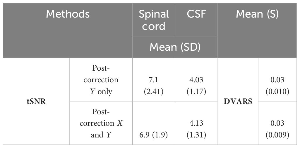
Table 1 Impact of Y-only vs. X and Y centerline correction on tSNR and DVARS.

Given these insights, we strategically focused on y-axis corrections for centerline realignment, aiming for an optimal balance between model performance and operational efficiency. This approach streamlined our procedures and reduced unnecessary computational expenditure, emphasizing our commitment to refining and improving our methodologies with a focus on cost efficiency and effectiveness (see Figure 1).

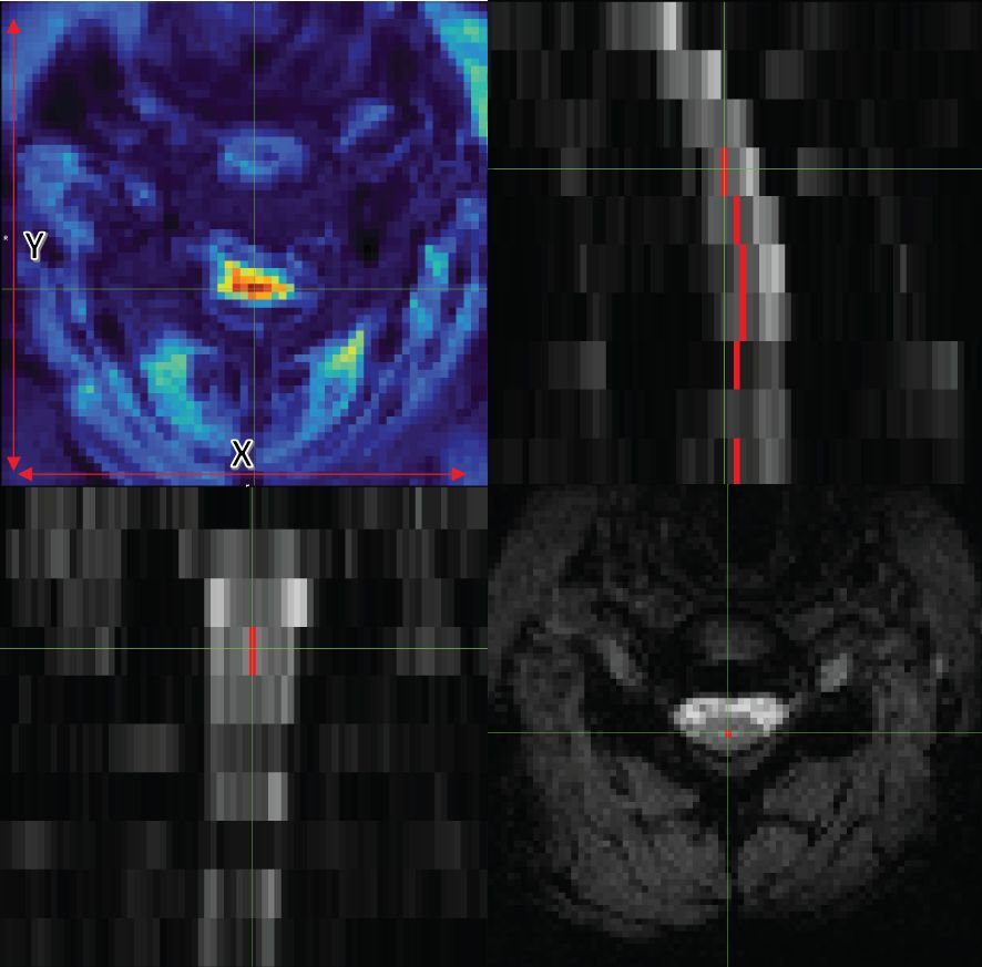
Figure 1 Axial (bottom right), coronal (bottom left), and sagittal (top right) views of data with the centerline. The image on the top left also shows tSNR with the x and y guidelines.

However, given that literature and empirical observations suggest minimal movement in the z-direction in spinal cord fMRI (36), we did not perform corrections in the z-direction. This targeted approach in preprocessing was designed to enhance the training efficiency and accuracy of our DeepRetroMoCo algorithm. Notably, the final output of DeepRetroMoCo’s spatial transformation map offers full freedom for correction across all considered directions, ensuring a comprehensive and effective motion correction for the entire dataset.

2.2 Unsupervised deep learning network architecture2.2.1 Convolutional neural network architecture

Assume M and F are two images of the same slice defined in the N-dimensional spatial domain Ω ⊂ RN. We are focusing on N = 2 because the type of data we are using is “functional,” containing single-channel grayscale data. Additionally, our network focuses on the Axial view. The fixed image F is the reference volume, so it can be the first, middle, average, or any of the volumes, and M is the rest of the time-series images. Before training the network, we align F and M using our fixing Centerline method, which we describe in the following section, so that the only misalignment between the volumes is nonlinear. We then use a CNN structure similar to UNet (37, 38) to model a Nθ (F,M) = Ø function, which includes an encoder and decoder with skip connection (Figure 2): where ∅ is the register map between the two input images and the θ learned parameter of the network. In this map, for each voxel p ∈ Ω, there is a position where F(p) and the warped image M(∅(p)) have the same anatomical position. Therefore, our network takes the concatenated images F and M as input and calculates the registration flow field based on θ. In the next step, it uses the spatial transformation operator to warp the moving image based on the flow field and evaluates the similarity between M and F and θ update. Figure 3 shows our introduced architecture and an integrated input by concatenating F and M in two channels of the 2D image.

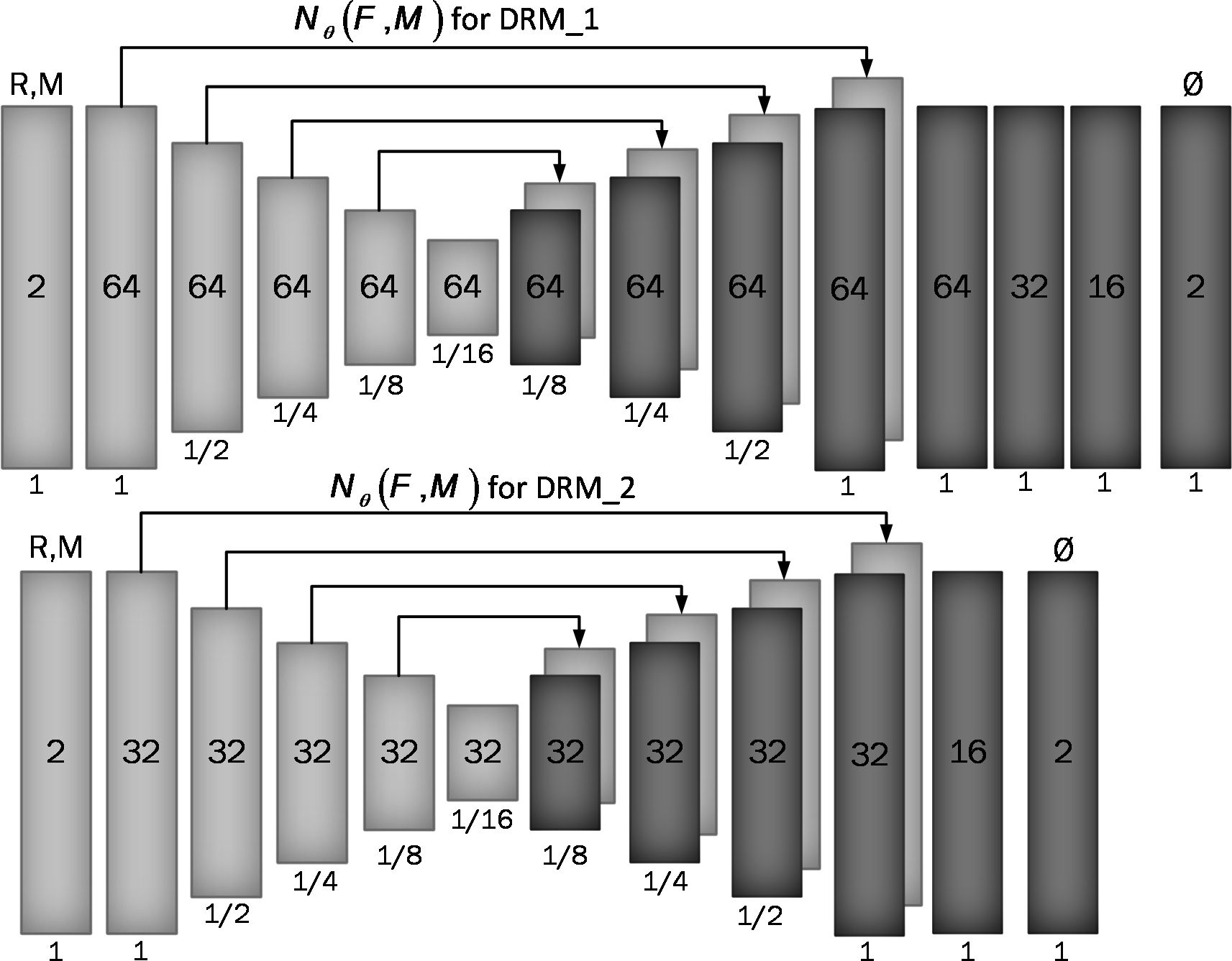
Figure 2 Proposed convolutional architectures implementing g_θ (F,M). Each rectangle shows a 2D volume in which two fixed and moving images are connected. The number of channels inside each rectangle is shown and the spatial resolution is printed below it according to the input volume. The first model has a larger architecture and more channels than the second model.

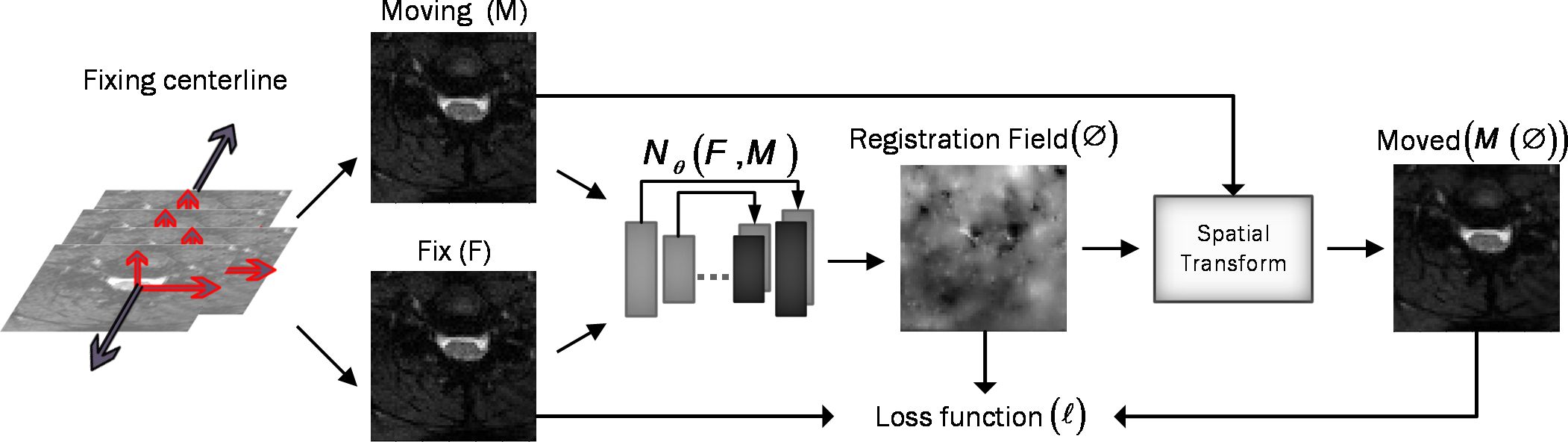
Figure 3 Overview of DeepRetroMoco. As a preprocess, we align the data in two dimensions based on the centerline, and then we register the moving image (M) to the fixed image (F) by learning function parameters (N). During training, an ST was used to warp the moving image with the registration field, and in this operation, the loss function compares M(Ø) and F using the smoothness of Ø.

In both the encoder and decoder stages, we use two-dimensional convolution with a 3×3 kernel size and leaky Relu activation. The hierarchical properties of the concatenated image pair are captured by the convolution layer, which is required to estimate ∅. We also use stride convolution to decrease the spatial dimensions and get to the smallest layer. During the encoding steps, features are extracted by downsampling, and during the decoding and upsampling steps, the network propagates the trained features from the previous step directly to the layer that generates the registry by using a skip connection. A decoder’s output size  (∅) is equal to the input image M.

We used two architectures to examine a trade-off between speed and accuracy. These two structures, DRM_1 and DRM_2, differ in their architectural complexity at the end of the decoder. DRM_1, being the more complex model, uses additional layers at the end of the decoder and more channels throughout, resulting in a total of 467,474 parameters. In contrast, DRM_2 is designed with fewer parameters, totaling 116,370, making it a more compact model. This difference in the number of parameters reflects the variations in computational complexity and capacity between the two models.

To find the optimal theta parameter, we used the stochastic gradient descent method to minimize the loss function ℒ: (Equation 1)

θ^=argminθ[E(F,M)∼D[ℒ(F,M,gθ(F,M))]](1)

where D is the empirical distribution. It should be noted that we do not need supervisor information such as Atlas or T1 images.

The ℒUnsupervised consists of two parts: (Equation 2) ℒsim, which measures the similarity between F and M(∅), and  ℒreg, which measures the smoothness of the registration field. Thus, our total loss function is as follows:

ℒ(F,M,∅)=ℒsim (F,M(∅))+λℒreg (∅)(2)

λ is the regulation parameter.

We used two different cost functions for ℒsim: mean square error (Equation 3) and normalize cross-correlation (Equation 4), which is a common metric due to robust intensity variations. The first cost function, the mean square error, is as follows:

MSE=1(Image sigma)2×1N×∑pi∈Ω(F(pi)−M(∅(pi)))2(3)

Here, pi is the position of the pixels and Image sigma is equal to 1 in this work. In addition, the fact that MSE is close to 0 indicates better alignment. The second cost function, normalizing cross-correlation, is as follows:

CC= ∑p∈Ω(∑pi(F(pi)−F^(p))(M(∅(pi))−M^(∅(p))))2(∑pi(F(pi)−F^(p)))(∑pi(M(∅(pi))−M^(∅(p))))(4)

Let F(pi) and M(∅(pi)) be the image intensities of fixed and moving images, respectively, and F^(p) and M^(∅(p)) be the local mean at position p, respectively. The local mean is computed over a local n2 window centered at each position p with n = 3 in this work.

By minimizing ℒsim, we seek to approximate M(∅(p)) from F(p), but it may cause a discontinuity in ∅, so we used spatial gradients to regulate the deformation field between the voxel’s neighborhood, as follows: (Equation 5)

ℒregularization =∑p∈Ω‖∇∅(p)‖2=∑‖∂∅∂x‖2+‖∂∅∂y‖2+‖∂∅∂z‖2  (5)

This cost function is applied to the network’s output vectors and controls the size of the vectors by deriving the vectors in each direction.

2.2.2 Spatial transformation function

Our spatial transformation function (STF) is critical for learning the transformation parameters θ, which align the moving image (M) with the fixed image (F) by minimizing their dissimilarity (39). This process is distinct from Pix2pix’s approach, which typically relies on paired examples in a supervised learning context for image-to-image translation. Our unsupervised method, instead, leverages the inherent structure within the data, learning θ directly from the alignment of M and F without the need for such pairs.

The STF generates a sampling grid using the predicted transformation parameters θ, creating a deformed version of M [notated as M(∅)]. It is worth noting that the STF in our network learns this deformation field in an unsupervised manner, which is not directly comparable to the Pix2pix model that requires paired training data. Moreover, our method uses bilinear interpolation at non-integer positions to ensure a smooth and continuous transformed image, which is critical for maintaining anatomical structure after transformation.

To further distinguish our work from Pix2pix, we use a unique loss function that balances the similarity between F and the warped image M(∅) with the regularization of the deformation field to ensure smoothness. This loss function is key for our network to produce a deformation field that enables precise alignment while preserving the structural integrity of the images.

2.3 Experiments2.3.1 Dataset

The data used for this experiment include 30 subjects with T2*-weighted MRI scans acquired from a 3T TIM Trio Siemens scanner (Siemens Healthcare, Erlangen, Germany) equipped with a 32-channel head coil, and a 4-channel neck coil was used for the imaging to investigate the functional activity in the brain and the spinal cord (40). All subjects were scanned twice. Five runs were collected in the first session and three runs were collected in the second session. Sessions were acquired 1 week apart. This resulted in 240 runs. We only used the data from the neck coil and cervical spinal cord in this study.

The dataset included 8–10 slices that covered the cervical spinal cord from C3 to T1 spinal segmental levels and were oriented parallel to the spinal cord at the C6 level. The FoV of the slices was 132×132 mm2, with voxel sizes of 1.2×1.2×5 mm3 and a 4-mm gap between them. The flip angle was 90°, and the bandwidth per pixel was 1,263 Hz, resulting in an echo spacing of 0.90 ms. 7/8 partial Fourier and parallel imaging (R = 2, 48 reference lines) was utilized again, resulting in a 43.3-ms echo train length and a 33-ms echo time. Finally, the TR for all slices was 3,140 ms, except for three subjects, who had TRs of 3,050 ms or 3,200 ms (depending on each participant’s coverage within the field of view). In the data preprocessing phase, we removed any instances of data that were deemed to be of low quality or exhibited discrepancies in data points when benchmarked against other datasets. Consequently, we curated a dataset comprising 27 subjects across 216 functional runs, of which 135 were allocated for the training set and the remaining 81 were allocated for the testing set. The training dataset was further partitioned into a 70:30 split for model training and validation, respectively. The validation subset played a crucial role in both the selection and performance evaluation of our proposed deep-learning models.

2.3.2 Evaluation

Since there is no gold standard for direct evaluation of functional registration or motion correction performance, we used two functional measures to check the signal strength of each subject or to examine signal variations in the group of volumes after predicting them by the network.

2.3.2.1 Temporal signal-to-noise ratio

Temporal signal-to-noise ratio (tSNR) is used to quantify the stability of the BOLD signal time series and is calculated by dividing the mean signal by the standard deviation of the signal over time (Equation 6).

tSNR=S¯σt_noise                             (6)

where S¯ is the mean signal over time and σ is the standard deviation across time. A better motion correction algorithm will result in greater tSNR values by reducing signal variations in the BOLD time series due to motion.

2.3.2.2 DVARS

DVARS (D, temporal derivative of time courses, VARS, variance over voxels) shows the signal rate changes in each fMRI data frame. In an ideal data series, its value depends on the temporal standard deviation and temporal autocorrelation of the data (41) and calculates the changes in the values of each voxel at each time point compared to its previous time point (42). DVARS was calculated in the whole image to find a metric that demonstrated the standard deviation of temporal difference images in the 4D raw data (43). DVARS was calculated using the following equation: (Equation 7)

DVARS(ΔI)i=(ΔIi(x))2=(Ii(x)−Ii−1(x))2 (7)

In this equation, ΔIi(x)  is used as local image intensity on the frame. DVARS could result in more accurate modeling of the temporal correlation and standardization because it is obtained by the most short-scale changes (41). The best value for this parameter is zero, and the closer it is to zero, the better the result.

We extracted the tSNR and DVARS parameters of output results by using the SCT toolbox and the FSL toolbox (44). For more accurate analysis of the tSNR parameter, we manually segmented the data into two parts, spinal cord and CSF, using the FSLeyes toolbox. Analyses compared the outcome of SCT and our method (DeepRetroMoco).

2.3.3 Statistical analysis

All statistical analyses were carried out using IBM SPSS Statistics (V. 25 IBM Corp., Armonk, NY, USA) with α< 0.05 as the statistical significance threshold. The Kolmogorov–Smirnov test was used to determine the normality of the parameters. For statistically significant results, the mean of normal data for each method was processed using one-way ANOVA with repeated measures in within-subjects comparison, followed by a multiple comparison post-hoc test with Bonferroni correction.

2.3.4 Implementation

In the course of our experiment, we evaluated our deep learning network’s performance both with and without the application of the “Fixing Centerline” preprocessing step. Our network underwent training over 200 epochs, each consisting of 150 iterations. The training process was executed using the Keras library with a TensorFlow backend (45) on an NVIDIA GEFORCE RTX 1080 GPU, which, on average, took 23 h to complete a full training cycle. To enhance our efficiency, we utilized the high-powered computational environment of Google Colab for model assessment and hyperparameter tuning, resulting in a more expedited analysis and learning process.

The optimization parameter we used was Adam, with a learning rate of 1e−4 (46). We trained our two models, the simpler DRM_2 and the more complex DRM_1, using two different cost functions, namely, normalized cross-correlation (NCC) and mean squared error (MSE), each with varying lambda values until convergence. Batch normalization was implemented to stabilize the training process, and min–max normalization was used during preprocessing to normalize the input data.

In our study, we designed an optimized data generator to deliver fMRI data to the network efficiently. This data generator operates by randomly selecting subjects and slices, ensuring that the training and validation sets are disjoint at the subject level. It then chooses a pair (fixed and moving images) from the corresponding volume, adhering to the specified batch size of 100 images. This approach of random selection at the subject level allows for the assessment of the model’s performance on new, unseen data, providing a robust evaluation of its noise-correction capabilities in a real-world setting where each subject’s data presents unique variations.

In comparison between the models, we chose the model that has better results in terms of our desired metric (tSNR) on the validation data. Then, we select one of the cost functions. Our code and model parameters are available online at https://github.com/mahdimplus/DeepRetroMoco.

3 Results3.1 Model selection

Table 1 displays the average of our method’s tSNR values in the validation data utilizing two distinct cost functions. The first model, DRM 1, outperforms DRM 2 in both Losses MSE and NCC by a slight margin. Furthermore, when the validation data of two cost functions in the first model are examined, NCC with an average of 10.13 ± 1 has better outcomes for the motion correction target based on the tSNR and statistical analysis, t(39) = 2.63, p< 0.05.

3.2 Visual comparison of motion correction protocols

Figure 4 presents a comparative evaluation of two motion correction techniques applied to fMRI data: sct_fmri_moco and Deepretromoco (DRM), juxtaposed with raw data. The results are demonstrated for a randomly selected subject at slice 4, with corrections displayed in two axes: the vertical (x-direction) and the horizontal (y-direction).

Figure 4 Comparative analysis of 3 protocols: SCT_fmri_moco (SCT), Deppretromoco (DRM), and raw data for Slice 4, showcasing precise centerline alignment across the x- and y-directions.

The center point on the reference volume, indicated on the figure, serves as the benchmark for evaluating the displacement of the centerlines across the volumes. The lines track the center points through subsequent volumes, highlighting the deviations from the reference.

In the vertical axis, the alignment of volume 94’s centerline with the reference illustrates the motion correction in the x-direction. The DRM method shows a fixed centerline, indicative of precise realignment, as opposed to the sct_fmri_moco method, where the centerline exhibits a discernible shift from the reference.

Conversely, in the horizontal axis, the alignment of the center points for volume 75 is examined. Here, the DRM method demonstrates a better match with the reference center point, suggesting a more accurate correction in the y-direction compared to the sct_fmri_moco method.

3.3 Statistical comparison of motion correction protocols

A one-way repeated-measures ANOVA was used to compare the influence of motion correction techniques on test data in sct_fmri_moco (12) and DeepRetroMoco, a deep neural network-based motion correction tool.

In a statistical comparison of tSNR parameters in the spinal cord, this parameter increased significantly from 7.104 ± 2.41 to 16.072 ± 3.09 arbitrary units (AU) (Table 2). Mauchly’s Test of Sphericity revealed that the assumption of sphericity had been violated, χ2(9) = 2.324, p< 0.313, and thus a Greenhouse–Geisser correction was used. The motion correction algorithm had a significant effect on the tSNR parameter in the spinal cord, F(2, 160) = 862.572, p< 0.0001. Post-hoc multiple comparisons using the Bonferroni correction revealed that the DeepRetroMoCo had a significantly higher mean tSNR in the spinal cord than the other motion correction method and raw data (p< 0.0001). Figure 5 depicts the significant difference between the groups using a violin plot.

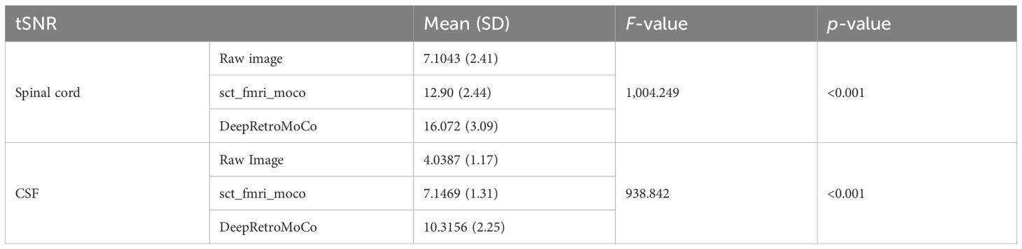
Table 2 Summary of tSNR as an image quality parameter between different motion correction methods (df = 4).

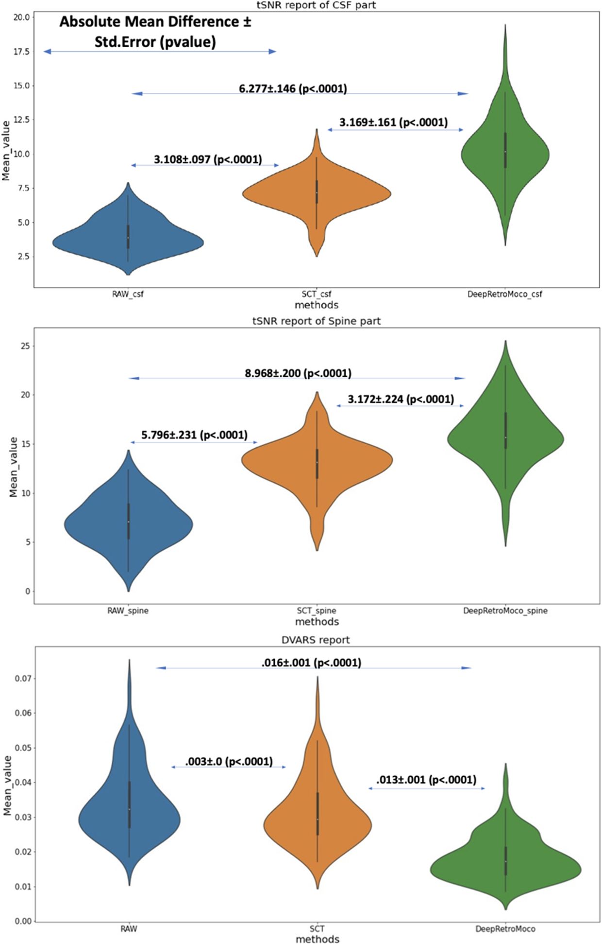
Figure 5 This figure depicts the mean and standard deviation of the SNR on the Spine and CSF sections (two top figures) that were manually segmented, as well as DVARS (bottom figure) with three types of results. RAW data that have not been corrected, SCT results, and DeepRetroMoco results are the three groups. The absolute mean difference + standard error (p-value) between groups is also reported. The mean difference is significant at the 0.05 level.

The tSNR in CSF increased significantly from 4.038 ± 1.17 to 10.315 ± 2.25 AU (Tables 2, 3). Mauchly’s Test of Sphericity revealed that the sphericity assumption had been violated, χ2(9) = 27.772, p< 0.0001, and thus a Greenhouse–Geisser correction was applied. The motion correction algorithm had a significant effect on the tSNR parameter in CSF, F(2, 160) = 949.72, p< 0.0001. Post-hoc multiple comparisons using the Bonferroni correction revealed that the DeepRetroMoCo’s mean tSNR in CSF was significantly higher than the other motion correction method and raw data (p< 0.0001) (Table 2). Figure 5 depicts the significant difference between the groups using a violin plot.

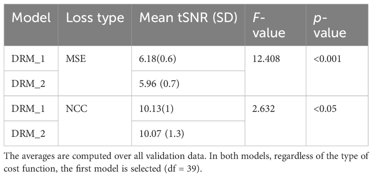
Table 3 Average tSNR for two types of our model, DRM-1 and DRM-2. Standard deviations are in parentheses.

DVARS decreased statistically significantly from 0.034 ± 0.009 to 0.018± 0.006 AU (Table 4). Mauchly’s Test of Sphericity revealed that the sphericity assumption had been violated, χ2(9) = 64.966, p< 0.0001, and thus a Greenhouse–Geisser correction was applied. The motion correction algorithm had a significant effect on the DVARS parameter, F(2, 160) = 309.349, p< 0.0001. Post-hoc multiple comparisons using the Bonferroni correction revealed that the DeepRetroMoCo had significantly lower DVARS than the other motion correction methods and raw data (p< 0.0001) (Table 4). Figure 5 depicts the significant difference between the groups using a violin plot.

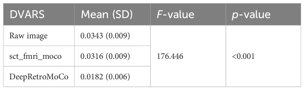
Table 4 Summary of DVARS as an image quality parameter between different motion correction methods (df = 4).

3.3.1 Reference volume impact on motion correction

To elucidate the impact of different reference volumes on motion correction efficacy in spinal cord fMRI, our study systematically evaluates first, mid, and mean volume references. Our findings, as depicted in Table 5, aim to establish a guideline for selecting the most effective reference volume to maximize motion correction accuracy, enhancing spinal cord fMRI