The relationship between heavy metals and metabolic syndrome using machine learning

1 Introduction

Metabolic syndrome (MetS) constitutes a conglomerate of disorders related to energy imbalance and metabolic dysfunction, predisposing individuals to cardiovascular diseases, diabetes, and subsequent complications, thereby elevating all-cause mortality rates and presenting a significant challenge to public health and socio-economic stability. By 2012, MetS had affected approximately one-third of the adult population in the united states (US), with a prevalence rate of 35% (1). The primary underlying mechanisms of MetS, attributed to an array of adverse lifestyle factors—including genetic predispositions, imbalanced nutritional intake, sedentarism, tobacco use, and alcohol consumption—entail the disruption of energy metabolism and the pathological accumulation of visceral fat (2–4). Moreover, environmental pollution has garnered considerable attention in recent research.

Growing epidemiological evidence suggests a link between heavy metal exposure and the risk of MetS and its components in the general population. For example, studies in Korean adults have shown that elevated blood levels of cadmium and lead correlate with a higher MetS risk, hinting at possible cumulative or synergistic effects among various heavy metals (5, 6). Nonetheless, some research has identified a negative or inverse relationship between heavy metal concentrations and MetS prevalence (7, 8). Compared to the general populace, individuals residing in heavy metal-contaminated areas—whether due to occupational or environmental factors—are at an increased risk of exposure through diverse pathways, which could affect the correlation between metal exposure and MetS risk. In Taiwan, particularly in industrial regions, there is a noted increase in MetS prevalence and blood glucose levels with rising arsenic exposure (9). Furthermore, MetS patients in areas endemic with arsenic-related diseases often report a history of consuming arsenic-laden water, and early arsenic exposure is linked to higher rates of hypertension and dyslipidemia (10, 11). While many studies have established a robust connection between chronic heavy metal exposure and Mets, the complex, nonlinear relationship between heavy metals and MetS complicates the use of traditional linear statistical methods. Moreover, epidemiological research frequently focuses on the effects of individual metals, neglecting the potential interplay among multiple metals and the common scenario of simultaneous exposure, which limits the ability to interpret complex health outcomes effectively.

To address this challenge, epidemiologists are increasingly adopting machine learning (ML) techniques known for their interpretability. Unlike traditional logistic regression, ML approaches offer several key advantages in the realms of medical research and healthcare applications (12). First, ML algorithms exhibit remarkable adaptability, adeptly managing complex, non-linear relationships among variables (13). This adaptability enables the detection of nuanced patterns and interactions within the data, enhancing prediction accuracy and overall model efficacy. Second, ML techniques generally exhibit greater resilience to outliers compared to logistic regression, managing extreme values with higher efficiency and less susceptibility to bias (14). Lastly, ML approaches enhance modeling of complex relationships in medical research and healthcare through their inherent flexibility, automation, and robustness (15).

In this study, we aimed to explore the associations between heavy metals and MetS using data from the National Health and Nutrition Examination Survey (NHANES, 2003–2018). We assessed nine ML models for their efficacy in detecting MetS from heavy metal exposure levels. Furthermore, we employed an advanced ML technique involving SHapley Additive exPlanations (SHAP) to shed light on the contribution of individual heavy metals to MetS detection. This methodology seeks to: (1) quantify the impact of each heavy metal on the ML models’ predictions; (2) explore the total effect of different heavy metals on metabolic syndrome and (3) enhance the development of early detection and intervention strategies specific to heavy metal exposure.

2 Materials and methods 2.1 Study population

The NHANES initiated in the early 1960s, is a comprehensive program aimed at evaluating the health and nutritional status of adults and children in the US. As a key initiative of the National Center for Health Statistics (NCHS), which is under the Centers for Disease Control and Prevention (CDC), NHANES uniquely integrates interviews with physical examinations to generate essential health statistics for the nation. Since 1999, NHANES has operated continuously, adapting its focus to address evolving health and nutrition issues and examining approximately 5,000 nationally representative individuals annually across various counties, with 15 counties selected each year (16).

The survey’s methodology includes both a detailed interview, covering demographic, socioeconomic, dietary, and health-related aspects, and a comprehensive examination that entails medical, dental, and physiological assessments, along with laboratory tests, conducted by skilled medical professionals. The selection process for NHANES is designed to reflect the demographic composition of the U.S. population, with particular emphasis on over-sampling older adults, African Americans, and Hispanics to ensure accurate and representative data.

Participants undergo a thorough examination by a physician, which includes dietary assessments and body measurements for all, blood sampling and dental screenings for most, and age-dependent tests and procedures. Data collection occurs in participants’ homes and in state-of-the-art mobile examination centers that are equipped to travel nationwide. The NHANES team, comprising physicians, technicians, and interviewers, utilizes advanced technology for data collection and processing, significantly reducing reliance on paper forms and manual coding.

Ethical approval for NHANES protocols was granted by the National Center for Health Statistics’ research ethics review committee, with all participants providing written informed consent.

For this analysis, we compiled NHANES data from 2003 to 2018, focusing on blood and urine metal levels and pertinent covariates, initially involving 80,312 participants. Exclusions were made for pregnant women or individuals under 20 years of age (32,723), those lacking heavy metal level data (33,120), and subjects with incomplete MetS information (3). Ultimately, 11,667 adults aged 20–79 were selected for the study. The selection process is illustrated in Supplementary Figure S1.

2.2 Data collection 2.2.1 Participant demographic data

Basic characteristics such as age, race, gender, family poverty to income ratio (PIR), education level, smoking and alcohol consumption were obtained through questionnaire surveys (17).

2.2.2 Analysis of heavy metals

In this study, 18 kinds of heavy metals in urine and blood were analyzed. All samples were collected during laboratory examination, and blood and urine samples were stored under appropriate freezing (−30 ° C) conditions until the day of detection. The whole blood and urine concentrations of heavy metals were determined by inductively coupled plasma mass spectrometry (ICP-MS) (16).

During the sample preparation phase of study, researchers subjected whole blood specimens to vortexing to achieve homogeneous distribution of cellular elements, followed by the extraction of a precise volume for metal concentration analysis. This procedure is pivotal, especially for metals predominantly located in red blood cells, such as lead, to ensure the representation of the specimen’s mean metal content. The addition of anticoagulants, notably ethylene diamine tetraacetic acid, is critical to prevent coagulation and preserve the uniformity of the sample, as coagulation can hinder the accurate sampling from the bulk specimen.

The dilution protocol preceding the analysis entails a standardized mixture of the sample with water and a specific diluent. This diluent comprises agents that liberate metals from red blood cells to facilitate ionization, mitigate ionization suppression, avert blockages due to biological matter, and incorporate internal standards to enhance analytical precision. Key diluent components, including Tetramethylammonium hydroxide and Triton X-100™, are instrumental in dissolving blood constituents and safeguarding the analytical instruments from contamination.

For the analytical phase, researchers employ an ICP-MS, which transforms liquid samples into aerosols, subsequently ionized within a plasma field, before their admission into the mass spectrometer. This stage demands meticulous temperature regulation and the application of internal standards to compensate for variations in the instrument’s performance. The spectrometer’s Dynamic Reaction Cell (DRC) is capable of operating in distinct modes, thereby amplifying specificity and sensitivity by diminishing interference, a crucial feature for analyzing elements like manganese, mercury, and selenium.

When the concentration of biomarkers is lower than the detection limit, the limit is divided by the square root of 2 according to NHANES scheme. See NHANES website for detailed determination methods. The NHANES quality assurance and quality control protocol meets the requirements of the clinical laboratory improvement act of 1988.

2.2.3 Ascertainment of outcomes

Metabolic syndrome can be diagnosed if the following ≥3 items are met (18):

1. Hypertension is systolic blood pressure ≥ 130 mmHg, diastolic blood pressure ≥ 85 mmHg, or has been diagnosed with hypertension and treated;

2. Fasting triglyceride ≥150 mg/dL, or the current use of drugs to treat high triglyceride;

3. Female HDL-c < 50 mg/dL, male hdl-c < 40 mg/dL, or the current use of drugs to reduce HDL;

4. Female waist circumference ≥ 88 cm, male waist circumference ≥ 102 cm;

5. Hyperglycemia is defined as fasting blood glucose ≥100 mg/dL or diabetes mellitus diagnosed and treated.

2.3 Data preprocessing and feature filtering

The data set was initially composed of 24 variables, called features in ML. It can be seen from Supplementary Tables S1, S2 that most of the data in this study sample are complete, and the missing data are less than 10%. According to the type of missing values, random forest filling method is used to deal with the missing data and the abnormal value is handled (Supplementary Tables S3, S4). The distribution of interpolated data is similar to the observed data (Supplementary Figure S2). In order to ensure that the data follow the normal distribution in the subsequent analysis, we performed logarithmic transformation on metal variables (Supplementary Table S5). Collinearity makes the parameter estimation of the model inaccurate, resulting in the model being too complex and over fitting the training data. We performed Pearson correlation analysis to test the relationship between these metals (Supplementary Figure S3). Using the least absolute shrinkage and selection operator (LASSO), the regularization term is introduced into the loss function to punish the model parameters and reduce the influence of collinearity. Variance inflation factor (VIF) is used to help identify the high correlation between independent variables, where VIF value below 10 indicates that there is no multicollinearity.

2.4 ML model strategies

The purpose of the multi-model classification approach is to identify the optimal model type, rather than to directly construct the final model. It employs a resampling mechanism (similar to k-fold) for training/validation to deduce the performance of each model (e.g., average AUC scores and variance) across multiple training sessions, focusing on the overall performance of each model category within the dataset. Then we will employ the best machine learning method for classification, with a total dataset sample size of N = 11,667, containing the following class information: Class (0): N = 7,827, Class (1): N = 3,840. From the total sample, a test set of N = 2,333 (20.00%) is randomly drawn, with the remaining samples used as a training set for 5-fold cross-validation. In this study, we used nine ML algorithms, namely extreme gradient boosting (xgboost) algorithm, logistic regression (LR), random forest (RF), AdaBoost, gaussian Nb (GNB), complementnb (CNB), multi-layer perceptron (MLP), and support vector machine (SVM) and k-nearest neighbor machine (KNN) learning models. See Supplementary Table S6 for specific parameters of each model. In order to further evaluate the predictive ability of the model for the final treatment results, the model was evaluated by area under the curve (AUC) value, accuracy, kappa coefficient, sensitivity, specificity, accuracy, recall rate, F1 and other indicators of the test data set (19).

SHAP additivity analysis is a method to explain individual prediction. It was originally evolved from the best Shapley value in game theory. The goal is to explain the prediction of instance X by calculating the contribution of each feature to prediction X. In this study, the algorithm is mainly used to sort according to the importance of variable characteristics in the model established by xgboost classifier, and screen out the top ten predictive factors in tb-dm patients. SHAP can reasonably explain the contribution value of each variable to the model, and avoid the long-standing “black box” theory in ML. Therefore, clinicians can make more optimal judgments when formulating treatment plans for patients (20).

2.5 Statistical analysis

In this study, continuous variables were expressed as mean ± standard deviation or interquartile interval (IQR; 25–75%). T test was used for normal continuous variables, while Mann Whitney U test was used for non-normal continuous variables. Categorical variables are described as percentages (%). Chi square or Fisher exact probability test is used for constituent ratio comparison. All statistical analyses were conducted using Python (version 3.10.9) and R software (version 4.2.3), with the Lasso R package glmnet at version 4.1.8, XGBoost in Python at xgboost = 2.0.1, and other methods in Python using scikit-learn = 1.1.3.The overall design of the paper is shown in Figure 1.

Figure 1. Model-making process and article framework. This figure shows how the data were obtained from electronic medical record systems, and the collection of data on all study variables, including demographic characteristics, laboratory indicators. Data on a total of 24 variables were collected, 22 of which were selected. The 22 variables were used to establish the machine learning models.

3 Results 3.1 Baseline data comparison

Table 1 presents the demographic characteristics of the study participants. A total of 11,667 individuals were included in the analysis, with 48.99% being male and an average age of 48.0 (interquartile range, 34.0–64.0). Out of the participants, 3,840 were diagnosed with MetS. Individuals with MetS tended to be older, have a higher body weight, be non-Hispanic white, and have a higher average family income (all p < 0.05). The content distribution of heavy metals in blood or urine in each two cycles from 2003 to 2018 is shown in Table 2.

Table 1. Characteristics of the study participants with and without MetS form 2003–2018 in US NHANES.

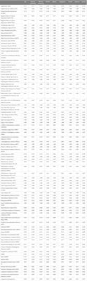
Table 2. Geometric means and geometric standard deviations of heavy metals by each cycle of US NHANES (2003–2018).

3.2 Feature selection

16 variables were selected using LASSO regression analysis based on their non-zero coefficients, as shown in Figure 2. These selected variables were blood cadmium, blood lead, blood mercury total, arsenous acid, arsenobetaine, arsenocholine, dimethylarsonic acid, barium, cadmium, cesium, lead, antimony, thallium, tungsten, uranium, molybdenum. The evaluation of multicollinearity among the various chosen metals and covariates using VIFs revealed no evidence of multicollinearity (Supplementary Table S7).

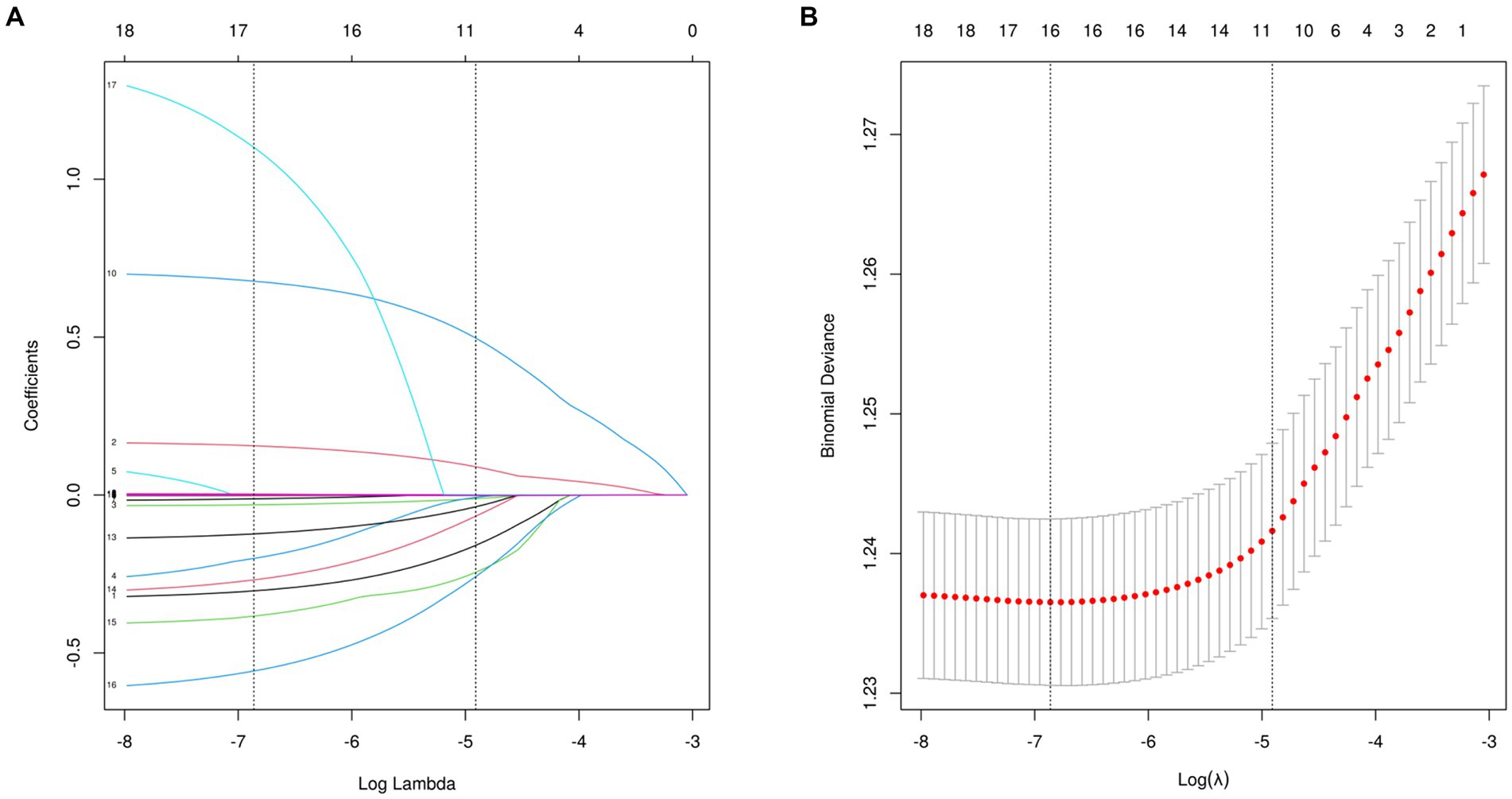
Figure 2. Features selection used the LASSO regression. (A) A coefficient profile plot is created against the logarithmic (lambda) sequence. In this study, the selection of predictors is based on the minimum criteria (indicated by the left dotted line), resulting in the selection of 16 nonzero coefficients using the LASSO regression model. (B) The tuning parameter (lambda) selection is based on the deviance in the LASSO regression, using both the minimum criteria (indicated by the left dotted line) and the 1-SE criteria (indicated by the right dotted line). LASSO, least absolute shrinkage and selection operator; SE, standard error.

3.3 Evaluation and comparison of the model

The AdaBoost model exhibited superior performance compared to other models, achieving a larger AUC as depicted in Figure 3 and Supplementary Table S8. Precision-recall curve are shown in Figure 4. A forest plot of the AUC score for the multiple models based on the AUC of the nine models was created (Figure 5), with the AdaBoost algorithm demonstrating the best predictive performance, achieving an AUC of 0.807. Since the performance of the validation set under the AUC index does not exceed the test set or the exceeding ratio is less than 10%, it can be considered that the fitting is successful (Figure 6). Consequently, the AdaBoost algorithm was chosen for further analyses. The training dataset values are presented in Table 3, and the validation set values are available in Table 4. Supplementary Figure S4 displays the confusion matrix for the nine ML algorithms used.

Figure 3. AUC curves for nine machine learning models. The AdaBoost model achieved a larger (better) AUC compared with the other models. (A) Training dataset (B) Validation dataset.

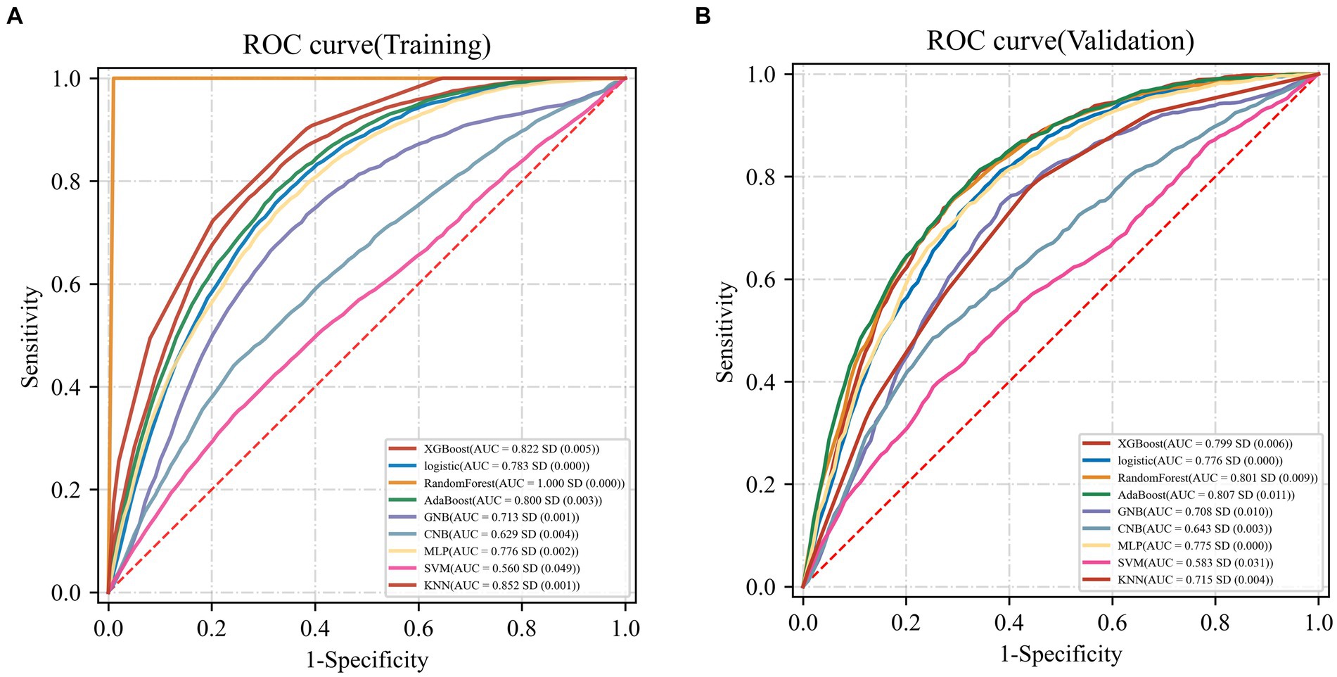
Figure 4. Precision-recall curve curves for nine machine learning models. (A) Training dataset (B) Validation dataset.

Figure 5. Forest plot of the AUC Score of the nine models. The AdaBoost model achieved a smaller (better) standard deviation (SD) compared with the other models.

Figure 6. AUC performance of training set and validation set.

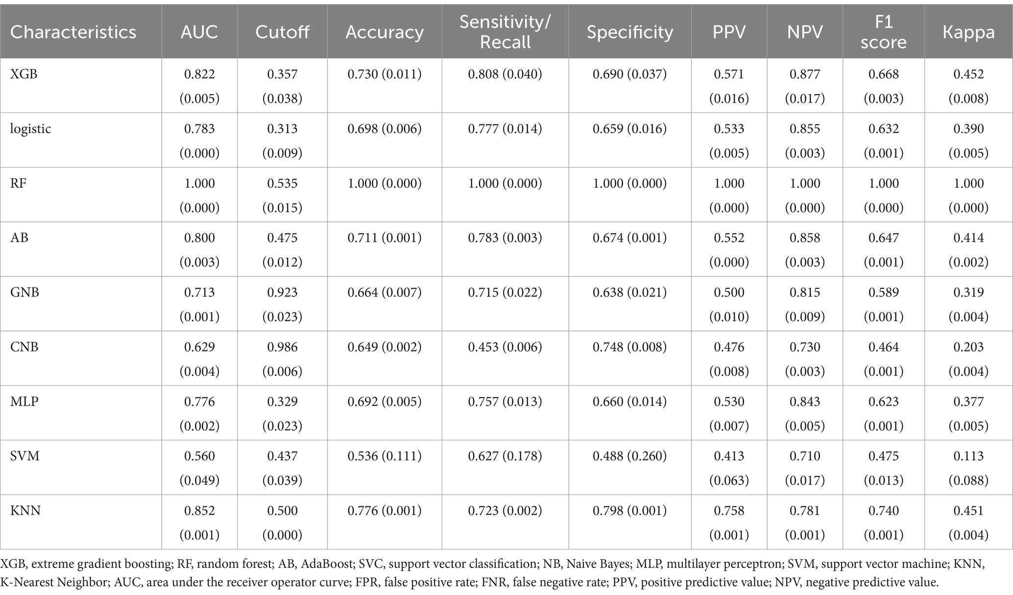
Table 3. Performance metrics for nine models in the training dataset.

Table 4. Performance metrics for nine models in the validation dataset.

3.4 Visualization of feature importance

After the above analysis, we use the SHAP method to explain the model established by AdaBoost. Figures 7, 8 shows the contribution of each screened feature to the model obtained by the SHAP method. Figure 8 offers an illustration of the assessment of MetS risk, showing the influence of features such as cadmium, body mass index (BMI), cesium, gender, and age on the estimated probability of MetS.

Figure 7. SHAP analysis of the AdaBoost model. (A) A visual representation of each feature of the AdaBoost model, showing the relationship between the importance of each feature. The color represents the value of the variable, with red representing the larger value and blue representing the smaller value. (B) The contributing variables are arranged in the horizontal line, sorted by the absolute value of their impact.

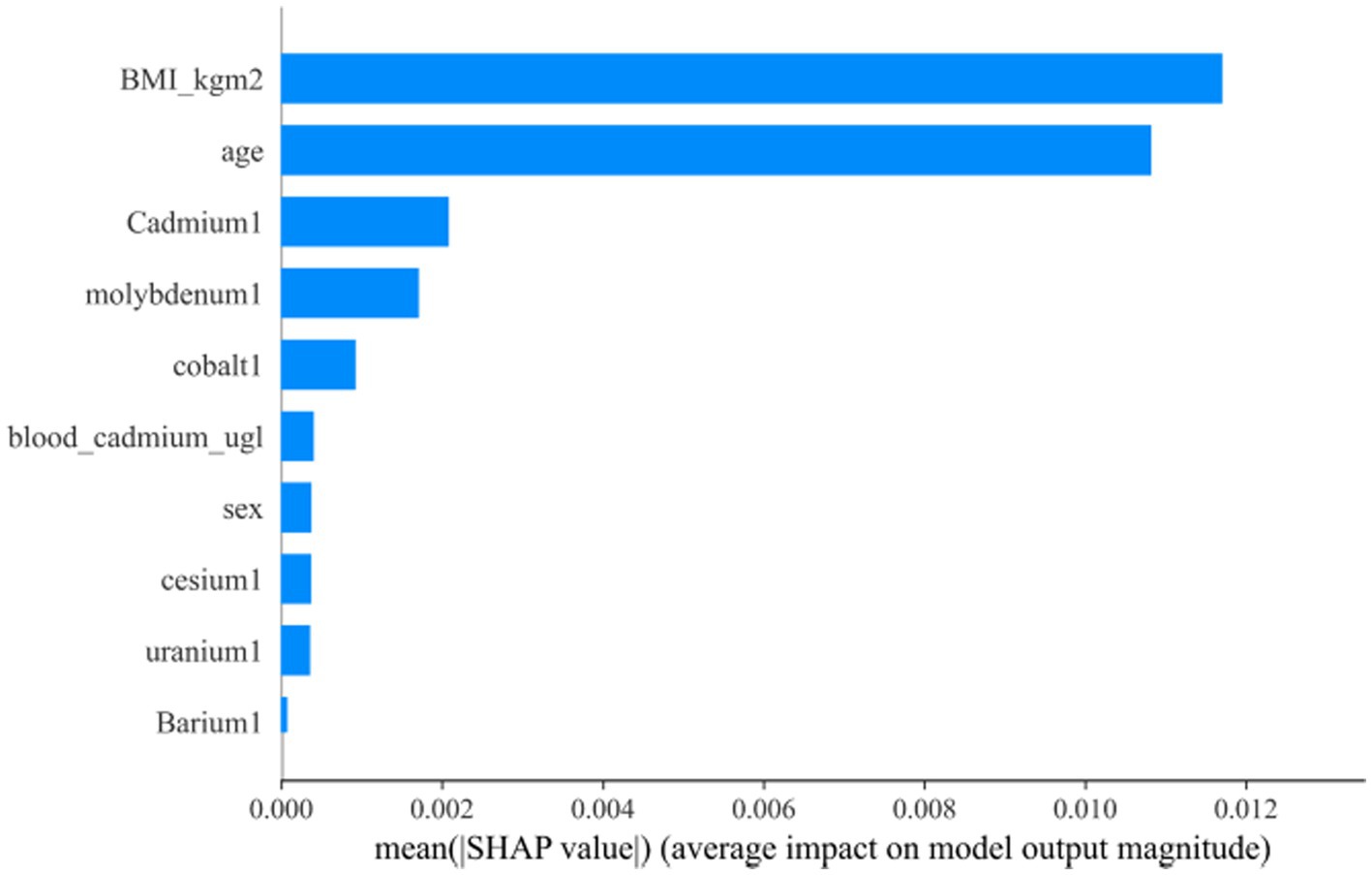
Figure 8. “SHAP” package to explain the importance of key variables to the model.

4 Discussion

In our study, we utilized a ML approach, complemented by an intuitive process, to investigate the relationships between heavy metal exposure levels and Mets. We developed nine ML models to detect MetS, achieving noteworthy predictive accuracy and interpretability from heavy metal datasets. The AdaBoost model, in particular, exhibited outstanding performance, pinpointing cadmium, molybdenum, cobalt, cesium, uranium, and barium as critical contributors to MetS detection. This ML model holds promise for supporting the creation of tailored healthcare strategies for individuals, based on their specific heavy metal exposure profiles.

This study extends previous work that employed ML algorithms for disease prediction, as demonstrated in several key studies (21–23). These investigations have underscored the capability of sophisticated classification algorithms to enhance prediction accuracy. In recent years, ML algorithms have increasingly contributed valuable insights to clinical decision-making processes. Leveraging vast clinical datasets, ML has rapidly advanced and proven its efficacy in forecasting the outcomes of various diseases (14). ML algorithms excel at synthesizing and analyzing large volumes of diverse data, a task that poses significant challenges for human analysts. Nonetheless, interpreting the outputs of ML algorithms remains complex (24). To address this complexity, we utilized SHAP values within the AdaBoost model to facilitate optimal interpretation and elucidate their influence on the predictive outcomes. In the context of the 2003–2018 NHANES survey, a positive SHAP value suggests that certain features elevate MetS risk, whereas a negative SHAP value indicates a lower risk.

This research revealed significant correlations between MetS and exposure to certain heavy metals, emphasizing the importance of recognizing the various dietary pathways through which these metals can be ingested. For instance, cadmium, commonly found in cereals, leafy vegetables, and shellfish, and chromium, present in meat, whole grains, and fruits, represent notable sources of exposure (25). Additionally, the consumption of fatty fish, dairy products, and meats may lead to exposure to Persistent Organic Pollutants (POPs), such as polychlorinated biphenyls (PCBs) and dioxins, which accumulate in the food chain and are associated with various negative health outcomes, including metabolic disorders (26–28). The identification of these heavy metals as factors contributing to MetS highlights the urgent need for comprehensive public health measures to mitigate exposure to these detrimental elements. Such measures could encompass policy-level initiatives to enforce stricter controls on industrial discharges and agricultural chemicals, alongside community and individual initiatives to enhance awareness of heavy metal and POP sources. Public health campaigns and dietary guidelines could also be instrumental in reducing consumption of contaminated foods. Furthermore, healthcare professionals have a pivotal role in screening for heavy metal exposure among susceptible groups and advising on dietary modifications to reduce such exposure.

The findings derived from SHAP analysis align with prior research outcomes. Specifically, Lee and Kim identified a notable positive association between blood cadmium levels and MetS risk in Korean males, utilizing data from the Korean National Health and Nutrition Examination Survey for the periods 2005–2010 and 2008–2012 (5, 29). Similarly, an Iranian study reported elevated urine cadmium levels in individuals with MetS (30). Additionally, experimental evidence revealed that serum chromium concentrations were lower in the diabetes group (0.0205 ± 0.0012 μg/mg) compared to the control group (0.0267 ± 0.0009 μg/mg). This finding was corroborated by Flores et al., who reported serum chromium levels in healthy individuals and diabetes patients to be 1.44 μg/L and 0.66 μg/L, respectively, further substantiating the observed disparity (31). From a mechanistic perspective, chromium enhances insulin sensitivity by activating insulin receptor kinase and facilitating insulin’s interaction with its cellular receptors, thus amplifying its biological efficacy.

Metals exhibit either additive or synergistic effects due to shared exposure routes and mechanisms of action, with oxidative stress being a principal shared pathway (32). Chronic exposure to heavy metals such as cadmium and lead results in glutathione depletion and the binding to sulfhydryl groups in proteins (33). The oxidation of Arsenite (As III) to Arsenate (As V) leads to the formation of hydrogen peroxide and the interaction with critical thiol groups (34). This cascade triggers an extensive production of free radicals, reactive oxygen species (ROS), and reactive nitrogen species (RNS), disrupting the balance within the antioxidant/oxidant system. The ensuing oxidative stress culminates in lipid peroxidation, Deoxyribo Nucleic Acid (DNA) and cellular membrane damage, protein alterations, and other detrimental effects, ultimately contributing to the onset of chronic conditions such as diabetes and cardiovascular diseases (35).

The AdaBoost model is distinguished by several key features. It leverages existing demographic, laboratory, and questionnaire data from the US NHANES, obviating the need for new data collection. This model integrates data from various sources to pinpoint the top 10 variables crucial for ML applications. Furthermore, between 2009 and 2013, heightened attention by the US government on heavy metal exposure, particularly in the context of environmental health, led to the initiation of numerous environmental governance initiatives (36). These initiatives resulted in reduced heavy metal levels and diverse MetS occurrences. Our ML models were developed and assessed using detailed participant data on blood heavy metal concentrations. Despite a general decline in heavy metal levels during 2009–2013, the NHANES dataset represents a single-time participation for individuals, implying that the heavy metal data does not reflect annual average exposure levels. However, this did not compromise the models’ stability, with the AdaBoost model demonstrating consistent reliability, indicated by an average AUC of 0.807. In addition to AdaBoost, we explored nine other ML techniques to detect MetS based on heavy metal exposure, drawing from recent cardiovascular disease research for enhanced insights. Certain models showed greater robustness and predictive accuracy with the incorporation of more granular data (37). An exhaustive evaluation of the ML models’ predictive capabilities revealed that the AdaBoost model stood out for its superior classification performance, underscored by nine distinguishing features.

This research presents novel insights, yet it is constrained by certain limitations that warrant acknowledgment. The cross-sectional nature of this study curtails the ability to establish causality or temporal sequences. Although the presence of heavy metals in biological specimens might indicate a connection with MetS or its constituents, the singular biomarker assessments in this study provide only a snapshot of exposure, with blood lead levels particularly reflecting recent exposures. Moreover, the dependence on self-reported data for MetS diagnosis in the US NHANES survey introduces a potential for information bias, including inaccuracies related to memory, which could affect the precision of the ML models in pinpointing MetS. The lack of an external validation group within our study design also limits the possibility of further substantiating the model’s reliability and its generalizability to a wider population.

Future research should emphasize the need for longitudinal studies to elucidate the causal connections between exposure to heavy metals and POPs and MetS. Exploring alternative biological matrices such as toenails or hair could provide more dependable indicators of long-term metal exposure, albeit with potential challenges related to measurement precision and varying growth rates. Subsequent inquiries should delve into the underlying mechanisms by which such exposures influence metabolic health, potentially through pathways like oxidative stress, inflammation, or hormonal disruption. A comprehensive understanding of the combined impacts of various metals and pollutants is crucial for developing effective prevention and intervention strategies. Expanding research to encompass diverse populations and settings will enhance the relevance and applicability of the findings, thereby informing public health initiatives tailored to the unique needs and risks of different communities. Furthermore, continuous analysis and interpretation of critical features will empower professionals with the insights necessary for informed decision-making, transcending mere dependency on algorithmic outputs. Efforts should also focus on validating the performance of models by enlarging the database and refining the interface between healthcare providers and ML models to improve their interpretability and practicality in clinical contexts.

5 Conclusion

In our study, the AdaBoost model exhibited exceptional effectiveness, precision, and resilience in identifying the association between heavy metal exposure and the incidence of MetS in participants from the US NHANES spanning 2003 to 2018. Employing transparent methods, we identified cadmium, molybdenum, cobalt, cesium, uranium, and barium as key contributors to the model’s predictive performance. Our results highlight the benefits of integrating machine learning approaches with SHAP techniques to explore the intricate impact of environmental exposures on health. Additionally, the predictive framework established by this research holds promise for devising targeted interventions to prevent and control MetS.

Data availability statement

The original contributions presented in the study are included in the article/Supplementary material, further inquiries can be directed to the corresponding authors.

Ethics statement

The ethics review board of the National Center for Health Statistics approved all NHANES protocols and written informed consents were obtained from all participants or their proxies (< 18 years). The study was performed in accordance with the ethical standards laid down in the 1964 Declaration of Helsinki and its later amendments. Bioethics Committee of Southern Medical University reviewed our study and have waived the need for ethical approval.

Author contributions

JY: Writing – original draft. ZD: Investigation, Software, Writing – original draft. FY: Formal analysis, Methodology, Writing – original draft. RD: Writing – review & editing. TF: Writing – review & editing.

Funding

The author(s) declare that no financial support was received for the research, authorship, and/or publication of this article.

Acknowledgments

Thanks to Jing Zhang (Shanghai Tongren Hospital) for his work on the NHANES database. His outstanding work, nhanesR package and webpage, makes it easier for us to explore the NHANES database. The manuscript has utilized written content generated or edited using a generative AI technology named “ChatGPT,” based on the GPT-4 architecture. GPT-4 stands for “Generative Pre-trained Transformer,” an advanced natural language processing model developed by OpenAI.

Conflict of interest

The authors declare that the research was conducted in the absence of any commercial or financial relationships that could be construed as a potential conflict of interest.

Publisher’s note

All claims expressed in this article are solely those of the authors and do not necessarily represent those of their affiliated organizations, or those of the publisher, the editors and the reviewers. Any product that may be evaluated in this article, or claim that may be made by its manufacturer, is not guaranteed or endorsed by the publisher.

Supplementary material

The Supplementary material for this article can be found online at: https://www.frontiersin.org/articles/10.3389/fpubh.2024.1378041/full#supplementary-material

References

3. Yao, F, Bo, Y, Zhao, L, Li, Y, Ju, L, Fang, H, et al. Prevalence and influencing factors of metabolic syndrome among adults in China from 2015 to 2017. Nutrients. (2021) 13:4475. doi: 10.3390/nu13124475

PubMed Abstract | Crossref Full Text | Google Scholar

5. Lee, BK, and Kim, Y. Blood cadmium, mercury, and lead and metabolic syndrome in South Korea: 2005-2010 Korean National Health and nutrition examination survey. Am J Ind Med. (2013) 56:682–92. doi: 10.1002/ajim.22107

PubMed Abstract | Crossref Full Text | Google Scholar

6. Rhee, SY, Hwang, YC, Woo, JT, Sinn, DH, Chin, SO, Chon, S, et al. Blood lead is significantly associated with metabolic syndrome in Korean adults: an analysis based on the Korea National Health and nutrition examination survey (KNHANES), 2008. Cardiovasc Diabetol. (2013) 9:9. doi: 10.1186/1475-2840-12-9

PubMed Abstract | Crossref Full Text | Google Scholar

7. Noor, N, Zong, G, Seely, EW, Weisskopf, M, and James-Todd, T. Urinary cadmium concentrations and metabolic syndrome in U.S. adults: the National Health and nutrition examination survey 2001-2014. Environ Int. (2018) 121:349–56. doi: 10.1016/j.envint.2018.08.029

PubMed Abstract | Crossref Full Text | Google Scholar

8. Rotter, I, Kosik-Bogacka, D, Dołęgowska, B, Safranow, K, Lubkowska, A, and Laszczyńska, M. Relationship between the concentrations of heavy metals and bioelements in aging men with metabolic syndrome. Int J Environ Res Public Health. (2015) 12:3944–61. doi: 10.3390/ijerph120403944