
記住我

The prediction of mortality in intensive care units (ICUs) helps to guide therapeutic decision making and resource allocation. It may also be useful for the counseling of family members and provision of prognostic information about critically ill patients.1 Several tools have been applied to predict the mortality of these patients; they include the Acute Physiology and Chronic Health Evaluation (APACHE) II,2 the Sequential Organ Failure Assessment (SOFA),3 and the Simplified Acute Physiology Score (SAPS) II.4 However, most such scoring systems were developed with Caucasian populations, and their accuracy when applied to Asian populations is unclear. Furthermore, these systems are based on traditional statistical techniques, with which the management of the abundance of data collected in the ICU is difficult, and do not utilize comprehensive patient information. In contrast, machine-learning techniques enable the analysis of complex signals in data-rich environments.5 This single-center study was conducted to develop a machine-learning model for the prediction of mortality in the very early stage of ICU admission using large-scale data collected from patients’ electronic medical records and by physiological monitoring. We hypothesized that the machine-learning model would be more accurate than traditional scoring systems.
2. METHODS 2.1. Study populationWe retrospectively screened the records and other data collected from all patients aged >20 years who were admitted to the medical and surgical ICUs of Taipei Veterans General Hospital from 2009 to 2018. The collected data included demographic characteristics, medical histories, vital signs, and laboratory findings from patients’ ICU stays. Philips IntelliSpace Critical Care and Anesthesia systems, which enable the collection of rich data about patients’ conditions streamed automatically from bedside monitors and input manually by health care providers, were used in the ICUs. These data included hemodynamic and ventilation parameters (e.g., from electrocardiographic monitors, pulse oximeters, and multiparameter monitors), nutrition prescriptions, information about medications administered, and regular notes from medical staff. We obtained data not recorded in the Intellispace Critical Care and Anesthesia systems (e.g., on medicines administered in the outpatient department and adverse events occurring after ICU discharge) from the hospital’s electronic medical records system. In order to address the missing values issue, an initial step involved the removal of features exhibiting a substantial proportion of missing data, specifically those with a missing rate exceeding 50%. Subsequently, for the remaining features, mean imputation was applied to continuous variables to fill in the missing values. Notably, the continuous variables which needed to impute missing fields, such as serum sodium, calcium concentrations, and central venous pressure, were Gaussian (normal) distribution. Additionally, no missing values were present in the categorical variables after eliminating features with high missing rates. All distributions of those features were symmetric, and the mean and median are all at the exact center value.
To evaluate disease severity, APACHE II2 and SOFA3 and SAPS II scores4 were calculated within 24 hour after ICU admission. The lowest mean arterial pressure and the highest heart rate (HR) within 24 h after ICU admission were recorded. The use of inotropes or vasopressors, such as norepinephrine and dopamine, was also recorded. White blood cell counts and blood chemistry studies were performed on ICU admission using routine laboratory methods. Sepsis was defined as organ dysfunction reflected by a ≥2-point increase in the SOFA score,3 consequent to infection.6 Shock was defined as hypotension requiring vasopressors to maintain a mean arterial pressure ≥65 mmHg and a serum lactate concentration >18 mg/dL, despite fluid resuscitation.6 For patients required mechanical ventilation, assist-control mode was used initially with a tidal volume 6 mL/kg ideal body weight, fraction of inspired oxygen (FiO2) 100%, and positive end expiratory pressure 5 to 8 cmH2O. The FiO2 would be adjusted hourly to achieve oxygen saturation (SpO2) 90 to 95% or partial pressure of oxygen (PaO2) 60 to 80 mmHg. The ventilator settings within first 24 hours of ICU admission were recorded and entered for analysis. This study was conducted according to the principles of the Declaration of Helsinki and was approved by the Research Ethics Committee of Taipei Veterans General Hospital (no. 2019-09-006BC), with waiver of the requirement for informed consent.
2.2. Development of machine-learning modelsWe used the extreme gradient boosting (XGBoost) and random forest (RF)7,8 ensemble methods to construct ICU mortality prediction models. XGBoost and RF are representative tree-based machine-learning methods. Training data were split into n subsets to build n trees (learners), and the results of the trees were then aggregated to generate the final results; in this way, many weak learners are incorporated to generate a strong learner. The difference between XGBoost and RF is the core algorithm. XGBoost is based on the boosting algorithm: given n subsets and n trees , Tk is trained on Sk, and the weights of the trained Tk are passed to Tk+1; in other words, a learner receives the learning results from the previous learner. RF is based on the bagging algorithm, which centers on “voting.” Tk is still trained on Sk, but the results are voted on by each Tk.
XGBoost and RF have shown remarkable performance in many classification tasks.9–12 One characteristic of these methods is the output of feature importance, which indicates the features or attributes that are the main factors affecting the classification. This output makes machine-learning models more explainable than models generated with deep-learning methods, which have been extensively used in many applications.13 However, only showing feature rankings is insufficient for deep analysis. Therefore, we applied SHapley Additive exPlanations (SHAP) values,14 which reflect the positive or negative influence of each feature in addition to its rank, for in-depth analysis and plotting. Thus, the feature ranking from top to bottom on the summary plots generated represents high to low degrees of significance for classification, and the SHAP values along the x axis represent positive and negative impacts on the models.
We obtained optimal hyperparameters for the models by grid search, selecting those with the best average results of k-fold cross validation (k=5) using different scoring methods. That is, in the training phase, we split the data into five folds and then took four folds as training data; one fold as validation data. Finally, the procedure was repeated five times. Specifically, the maximum depths of RF configurations 1 and 2 were 13 and 26, and the corresponding maximum features were 16 and 19, respectively. For XGBoost, configurations 1 and 2 had the same gamma and scale_pos_weight values (5 and 2, respectively), and maximum depths of 2 and 3, respectively. Default values were used for the remaining hyperparameters. Details of the settings for the two XGBoost configurations are provided in the Additional files: https://links.lww.com/JCMA/A234.
2.3. Statistical analysisThe enrolled patients were allocated to training (n = 9901) and testing (n = 2476) datasets. The data of two datasets were compared using the Mann–Whitney U test for continuous variables (expressed as medians and interquartile ranges), and Fisher’s exact test for categorical variables (expressed as counts and percentages). Areas under receiver operating characteristic curves (AUCs) were used to evaluate the accuracy of the severity scores and machine-learning models in predicting mortality of critically ill patients. The accuracy (ACC), positive predictive value (PPV), and negative predictive value (NPV) of each model were calculated. To investigate the performance of machine-learning models modified by varying conditions, we performed subgroup analyses with the cohort stratified by patients’ age, APACHE II scores, SOFA scores, and the usage of mechanical ventilator. In addition, we performed logistic regression analysis to confirm the independence of clinical variables composed the machine-learning models. The five most predictive variables used in RF and XGBoost models were further adjusted in multivariate logistic regression analysis. The analyses were performed with SPSS (ver. 18.0; SPSS Inc., Chicago, IL, USA) and SAS (ver. 9.3; SAS Institute Inc., Cary, NC, USA). A p value < 0.05 was considered to indicate significance.
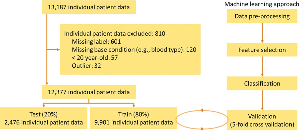
3. RESULTS 3.1. Sample characteristicsOf 13,187 cases screened, data from 810 patients aged <20 years or with missing labels were excluded, leaving a sample of data from 12,377 patients. A flowchart of patient enrollment and classification is provided as Fig. 1. The distributions of age, sex, comorbidities, medications administered, disease severity, vital signs, and laboratory results were similar between the training and testing datasets (Table 1). The median age of the enrolled patients was 70.0 years, and 7966 (64.36%) patients were male. In total, 8360 (67.54%) of the patients were admitted to the medical ICUs (ICU-A and ICU-C) and 4017 (32.46%) patients were admitted to the surgical ICU (ICU-B). In medical ICUs, the highest proportion of patients’ subspecialties was the division of hematology and oncology (20.0%), followed the divisions of infectious diseases (14.9%), gastroenterology (13.3%), and nephrology (8.4%). The most common reasons for patients admitted to the medical ICUs were acute respiratory failure (44.1%), shock (21.8%), and acute renal failure (14.1%). On the other hand, the highest proportion of patients’ subspecialties in the surgical ICU was the division of general surgery (31.1%), followed the divisions of colorectal surgery (15.4%), transplantation surgery (14.2%), and oral and maxillofacial surgery (8.7%). The most common reasons for patients admitted to surgical ICU were intensive care after major surgery (53.3%), acute respiratory failure (18.8%), and shock (18.1%). In the medical and surgical ICUs, 9210 (74.41%) patients were under mechanical ventilation and 3327 (26.88%) patients were under vasopressor (norepinephrine) treatment. The median APACHE II score of the study population was 23.5. Details of the sample characteristics are provided in Supplementary File 1, https://links.lww.com/JCMA/A234.
Table 1 - Summary of patients’ baseline characteristics TotalALT=alanine aminotransferase; AST=aspartate aminotransferase; BT=body temperature; COPD=chronic obstructive pulmonary disease; CRP=C-reactive protein; CVP=central venous pressure; DBP=diastolic blood pressure; eGFR=estimated glomerular filtration rate; FiO2= fraction of inspired oxygen; GCS=Glasgow Coma Scale; GI=gastrointestinal; HCO3=bicarbonate; ICU=intensive care unit; I/O=intake/output; PaCO2=partial pressure of carbon dioxide; PaO2=partial pressure of oxygen; PEEP=positive end expiratory pressure; SBP=systolic blood pressure; UO=urine output; WBC=white blood cells.
 Fig. 1:
 Flowchart of patient enrollment and classification.
3.2. Performance of machine-learning models and traditional scoring systemsReceiver operating characteristic curves characterizing the ability of the different models to predict ICU mortality are presented in Fig. 2, and corresponding c-statistics are provided in Table 2. The XGBoost model had the greatest area under the curve (AUC 0.880, sensitivity 0.802, specificity 0.805; ACC 0.874, PPV 0.619, NPV 0.921), followed by the RF model (AUC 0.876, sensitivity 0.815, specificity 0.777; ACC 0.871, PPV 0.621, NPV 0.911). In contrast, SOFA scores (AUC 0.747, sensitivity 0.815, specificity 0.549; ACC 0.592, PPV 0.258, NPV 0.939), SAPS II scores (AUC 0.743, sensitivity 0.872, specificity 0.462; ACC 0.528, PPV 0.237, NPV 0.950), and APACHE II scores (AUC 0.738, sensitivity 0.820, specificity 0.505; ACC 0.556, PPV 0.241, NPV 0.936) had much smaller AUCs and less specificity. Table 3 shows the 5-fold cross-validation results, and it demonstrates that XGBoost with AUC 0.900 (95% CI, 0.893-0.907), sensitivity 0.806, and specificity 0.829, which outperformed the performance of conventional scoring systems (relative increase of 18% in AUC).
Table 2 - C-statistics for models for the prediction of mortality in the intensive care unit (testing database) Method AUC Sensitivity Specificity ACC PPV NPV Random forest (config. 1) 0.876 0.805 0.798 0.868 0.596 0.918 Random forest (config. 2) 0.876 0.815 0.777 0.871 0.621 0.911 XGBoost (config. 1) 0.880 0.802 0.805 0.870 0.598 0.922 XGBoost (config. 2) 0.880 0.802 0.792 0.874 0.619 0.921 SOFA score 0.747 0.815 0.549 0.592 0.258 0.939 SAPS II score 0.743 0.872 0.462 0.528 0.237 0.950 APACHE II score 0.738 0.820 0.505 0.556 0.241 0.936ACC=accuracy; AUC=area under the ROC curve; APACHE II=Acute Physiology and Chronic Health Evaluation II; NPV=negative predictive value; PPV=positive predictive value; SAPS II=Simplified Acute Physiology Score II; SOFA=Sequential Organ Failure Assessment; XGBoost=extreme gradient boosting.
ACC=accuracy; AUC=area under the ROC curve; APACHE II=Acute Physiology and Chronic Health Evaluation II; NPV=negative predictive value; PPV=positive predictive value; SAPS II=Simplified Acute Physiology Score II; SOFA=Sequential Organ Failure Assessment; XGBoost=extreme gradient boosting.
 Fig. 2:
 Pairwise comparison of ROC curves for the models for the prediction of mortality in intensive care units. APACHE II=Acute Physiology and Chronic Health Evaluation II, AUC=areas under ROC curve, RF=random forest; ROC=receiver operating characteristic, SAPS II=Simplified Acute Physiology Score II, SOFA=Sequential Organ Failure Assessment, XGBoost=extreme gradient boosting.
3.3. Feature importance and independence of variables in the machine-learning modelsThe variables used in the machine-learning models and their relative importance are shown in Figs. 3 and 4. The hyperparameters and setting details for the two XGBoost configurations are provided in Supplementary Files 2 and 3, https://links.lww.com/JCMA/A234. Norepinephrine usage in the ICU, the FiO2, the lowest and highest of Richmond Agitation and Sedation Scale (RASS) scores, and prothrombin time (PT) were the five most predictive variables in the RF models. Twenty-four-hour urine output, FiO2, PT, HRs, and platelets were the five most predictive variables in the XGBoost models. Above variables were all significantly associated with of ICU mortality in the univariate logistic regression analysis. In the multivariate logistic regression analysis, norepinephrine usage, FiO2, the highest RASS scores, PT, 24-hour urine output, HRs, and platelets were still independently associated with the incidence ICU mortality (showed in Table 4).
Table 4 - Univariate and multivariate logistic regression analysis to interpret the association between ICU mortality and clinical variables in machine-learning models Univariate Multivariate* Crude OR (95% CI) p Adjusted OR (95% CI) p Usage of norepinephrine 0.154 (0.083-0.288) <0.001 0.333 (0.143-0.772) 0.010 FiO2 1.055 (1.037-1.074)
留言 (0)