Animals

We selected male Sprague–Dawley (SD) rats aged 7–8 weeks old and weighing 250 ± 20 g (the Animal Center of Fuwai Hospital). All experimental protocols were approved by Fuwai Hospital Animal Experimental Committee. All experimental rats were housed three per cage under the environment 22 °C with a 12-h light/dark cycle and had ad libitum access to food and water for 7 d to adapt to the new environment.

Hematoxylin–eosin (HE) staining

The brain tissues of rats (Procedure A) on the day 22 were collected, fixed in 4% paraformaldehyde, embedded in paraffin, and dissected into sections with 10 μm thickness. Each section was then deparaffinized, hydrated, washed, and stained with hematoxylin–eosin (H&E) using a commercially purchased kit (Beyotime, Shanghai, China).

Experimental design

In the current study, all rats were randomly assigned into two procedures after 7 days adaptation (Fig. 1). In Procedure A, the rats were divided into three groups.1) Normal(A1) group (n = 4): non-CUS and non-cardiac surgery; 2) cardiac surgery (A2) group (n = 4): non-CUS but cardiac surgery; and 3) CUS and cardiac surgery (A3) group (n = 4). As the Fig. 1B shows, the rats were randomly divided into three groups in procedure B.1) control (B1) group (n = 6): non-CUS and non-cardiac surgery; 2) cardiac surgery (B2) group (n = 6): non-CUS but cardiac surgery; and 3) CUS and cardiac surgery (B3) group (n = 10): CUS and cardiac surgery. The objective of establishing the cardiac surgery group is to eliminate the impact of acute stress induced by cardiac surgery on the rats. Meanwhile, the purpose of the control group is to mitigate the influence of confounding factors on the experiment. The rats assigned to the groups of non-CUS were kept undisturbed in their own cages, while rats assigned to the CUS group were exposed to chronic unpredictable stress for 21 days. The weights of rats were meticulously recorded on day 0, 7, 14, and 21. A comparative analysis of weight, using the Welch t-test, was conducted on days 0 and 21 between rats exposed to CUS and those in the non-CUS group to confirm the stress level of CUS rats [18]. On day 22, We performed cardiac surgery on cardiac surgery groups and decapitated all rats immediately after surgery. We isolated the whole rats’ brain for HE staining in procedure A and isolated the rats’ hippocampus for data-independent acquisition (DIA) and untargeted metabolomics in procedure B.

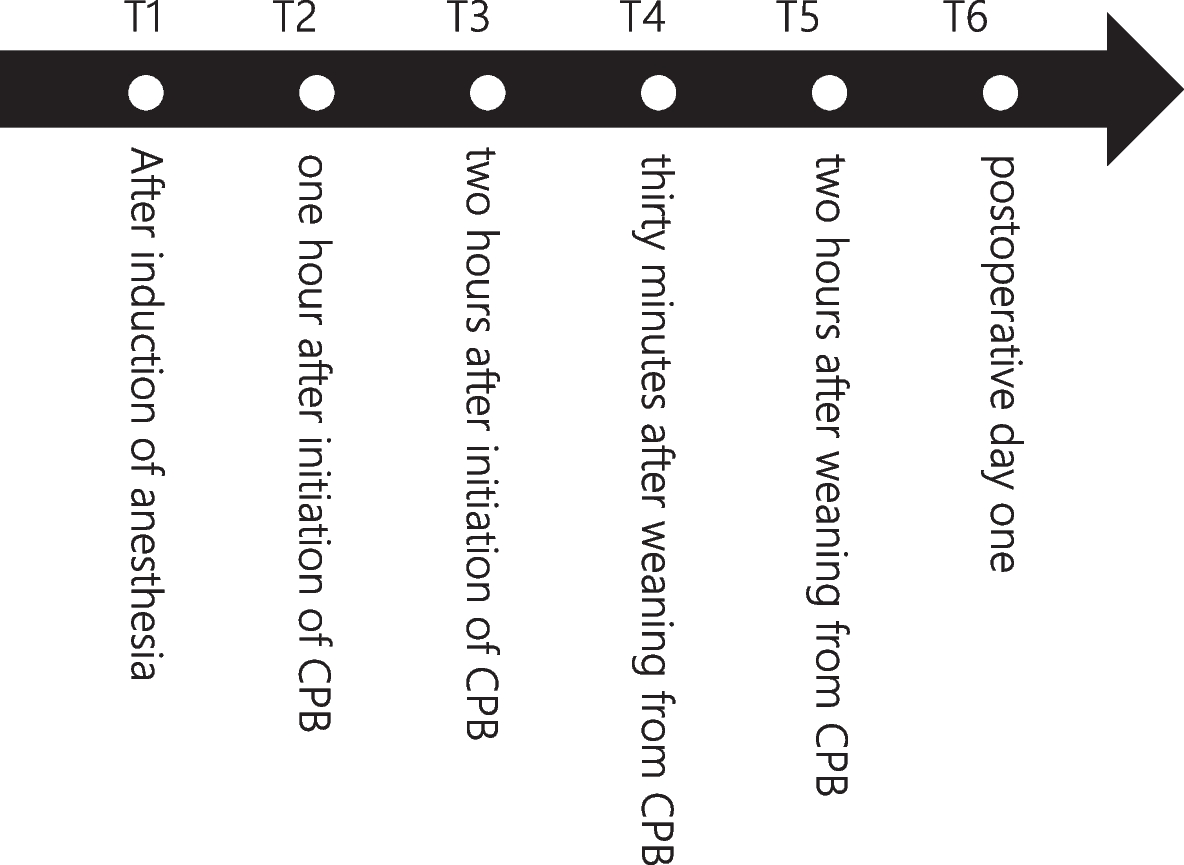
Fig. 1

Experiment Timeline (A) Procedure A (B) Procedure B

Chronic unpredictable stress (CUS) model

Rats assigned to the CUS groups were exposed to two of the following eight stressors daily for consecutive 21 days: 1) 40 Hz 90 dB noise stimulation for 9 min; 2) swimming for 5 min in 4℃ cold water; 3) body restraint for 1 h; 4) pinching tail for 1 min; 5) food deprivation for 24 h; 6) water deprivation for 24 h; 7) nyctohemeral rhythm inversion, and 8) cage tilt at 45º [19]. To prevent the rats from adapting to the stress factors, we exerted two different stress factors on them daily, and the stressors varied within 48 h [19]. We performed the cardiac surgery under cardiopulmonary bypass (CPB) on day 22.

Cardiac surgery model under cardiopulmonary bypass (CPB)

According to the surgical protocol from Koning et al. [20], the rats were anesthetically induced by 5% isoflurane inhalation and had no foot reduction response under pain stimulation, followed by endotracheal intubation (16G), and mechanical ventilation (tidal volume: 10 ml/kg, respiratory rate: 60–65 breaths/min, peep 2-4cmH2O). 2–3% isoflurane was continuously inhaled to maintain anesthesia and intraoperative inhaled oxygen concentration was 35%. The body temperature was maintained at 36.5℃ except during extracorporeal circulation. The blood pressure of the tail artery was monitored with a 22-G cannula needle. Fentanyl was 12 μg/kg, the intravenous injection was repeated before the start of CPB and 40 min after CPB, and inhaled isoflurane concentration was reduced to 1.5–2% when fentanyl was injected. The main components of CPB include a venous blood reservoir, a transfer pump, and a 4 ml oxygenator heat exchanger with three layers of hollow fiber membrane. Pipe through the right femoral artery and right jugular vein, and the end of the right jugular vein reaches the right atrium. After 500 U / kg of intravenous heparin, CPB was initiated and lasted for 30 min. The heart was exposed during CPB. Blood gas and hemoglobin concentrations were monitored at 10 min and 30 min after the start of CPB, and at 10 min and 60 min after the end of CPB, respectively. The pump liquid of CPB was 10 ml of 6% hydroxyethyl starch with a flow rate of 150–200 ml/kg/ min. The body temperature was maintained at the level of mild body hypothermia (35℃) during CPB and rewarmed slowly to 36–36.5℃, and then CPB was halted. Mechanical ventilation was restarted 10 min before the end of CPB. Heparin was neutralized by 2 mg/kg of protamine within 15 min after the end of CPB.

Immediately after surgery, when is the most severe brain injury occurs [12], all rats were decapitated, and the whole hippocampal tissue of the brain was isolated and frozen in liquid nitrogen, and then transferred to the fridge at -80 ℃.

Data-independent acquisition (DIA) proteomics analysisTotal protein extraction and sample preparation

Hippocampal tissue (Procedure B) was ground individually in liquid nitrogen and lysed with lysis buffer containing 8 M Urea, 100 mM NH4HCO3 (pH 8), and 0.2% SDS, followed by 5 min of ultrasonication on ice. The lysate was centrifuged at 12000 g for 15 min under the 4℃ environment and the supernatant was transferred to a clean tube. Extracts from each sample were reduced with 10 mM DTT for 1 h at 56℃ and subsequently alkylated with sufficient iodoacetamide for 1 h at room temperature in the dark. Then samples were completely mixed with 4 times the volume of precooled acetone by vortexing and incubated at -20℃ for 2 h or more. Samples were then centrifuged, and the precipitation was collected. After washing twice with cold acetone, the pellet was dissolved by dissolution buffer, which contained 0.1 M triethylammonium bicarbonate (TEAB, pH 8.5) and 6 M urea.

To perform protein quality test, the BSA standard protein solution was prepared according to the instructions of Bradford protein quantitative kit, with gradient concentration ranged from 0 to 0.5 g/L. The standard curve was drawn with the absorbance of standard protein solution and the protein concentration of the sample was calculated. Then 120 μg of each protein sample was taken and the volume was made up to 100 μL with dissolution buffer, 1.5 μg trypsin and 500 μL of 100 mM TEAB buffer were added, after one night digestion, supernatant was collected and washed with washing buffer for 3 times,the eluent of each sample were combined and lyophilized.

LC–MS/MS analysis and data analysis

According to the protocol provided by Novogene,the sample was fractionated using a C18 column (Waters BEH C18 4.6 × 250 mm, 5 μm) on a Rigol L-3000 HPLC system. Proteomics analyses were conducted utilizing the EASY-nLC™ 1200 UHPLC system (Thermo Fisher), coupled with a Q Exactive HF-X mass spectrometer (Thermo Fisher). The instrument operated in both data-dependent acquisition (DDA) mode and data-independent acquisition (DIA) mode, each applied separately.

The protein database employed Proteome Discoverer 2.4 (PD2.4, Thermo) to analyze data obtained through DDA scanning. Key search parameters included a 10 ppm mass tolerance for precursor ions and a 0.02 Da tolerance for fragment ions. Fixed modifications comprised cysteine alkylation, while variable modifications encompassed methionine oxidation and N-terminus acetylation, allowing for up to 2 missed cleavage sites. To improve analysis quality, PD2.4 filtered results, retaining only peptide spectrum matches (PSMs) with a confidence level exceeding 99% and proteins with at least one unique peptide segment. False discovery rate (FDR) validation removed PSMs and proteins with FDR greater than 1%.

Identification outcomes from PD2.4 were imported into Spectronaut (version 9.0, Biognosys) to generate a spectral library. Peptide and ion pair selection rules were applied [21], choosing peptides and sub-ions meeting criteria to form a target list. DIA data was then imported, with chromatographic peaks extracted based on the target list. Sub-ion matching and peak area calculations enabled simultaneous qualitative and quantitative analysis of peptide segments. Retention time calibration used standard peptides in the samples, and a precursor ion Q-value cutoff was set at 0.01.

Differential protein analysis

The identified proteins were annotated by the databases of Cluster of Orthologous Groups of proteins (COG), Gene Ontology (GO), KEGG (Kyoto Encyclopedia of Genes and Genomes), and IPR [22]. Quantitative analyses of proteins included total differential analysis of identified proteins, screening and expression pattern clustering analysis of the differential proteins. The progress of protein differential analysis included: 1) picking out the sample pairs for comparison; 2) calculating fold change (FC): the ratio of the mean of all biological repeat quantitative values of each protein in the comparison sample pair. To determine the significance of the difference, a Welch t test of relative quantitative values of each protein in the sample and the corresponding p-value was calculated as a significance indicator. Up-regulation protein was screened when the p-value <0.05, meanwhile FC 1.2 or more, while down-regulation was screened when the p-value <0.05, meanwhile FC 0.83 or less based on previous research [23, 24]. After that, we conducted GO and KEGG functional enrichment analysis to observe the function of selected differential proteins [25].Then, we performed subcellular localization analysis to examine the spatial expression patterns of differentially expressed proteins (DEPs).Finally, the probable protein–protein interaction were predicted using the STRING-db server [26].

Untargeted metabolomicsSample preparation

Samples (100 mg each) were extracted and grounded with liquid nitrogen individually, and the homogenate was resuspended by a well vortex on ice with precooled buffer (80% methanol and 0.1% formic acid). The supernatant of the lysate was diluted to the final concentration by LC–MS grade water after centrifugation at 15,000 g at 4 °C for 20 min. The samples were transferred into a new tube and were centrifuged at 15,000 g at 4 °C for 20 min, and the supernatant was subsequently injected into the LC–MS/MS system analysis [27].

UHPLC-MS/MS analysis and data processing

Samples were loaded using a Hypesil Gold column (100 × 2.1 mm, 1.9 μm) on a Vanquish UHPLC system (Thermo Fisher, Germany) coupled with an Orbitrap Q ExactiveTMHF-X mass spectrometer (Thermo Fisher, Germany) in Novogene Co., Ltd. The stated linear gradient was 17 min and the flow rate was 0.2 ml/min.

For the data process, the raw data files generated by UHPLC-MS/MS were processed using the Compound Discoverer 3.1 (CD3.1, ThermoFisher) to perform peak alignment, peak picking, and quantitation for each metabolite. The primary parameters were configured as follows: a retention time tolerance of 0.2 min, an actual mass tolerance of 5 ppm, a signal intensity tolerance of 30%, a signal-to-noise ratio of 3, and a minimum intensity threshold of 100,000. After that, peak intensities were normalized to the total spectral intensity. Following this, the intensities of peaks were adjusted to the total spectral intensity. The resulting normalized data was then employed to forecast the molecular formula using information from additive ions, molecular ion peaks, and fragment ions. And then peaks were matched with the mzCloud (https://ww.mzcloud.org/). mzVault and MassList database to obtain the accurate qualitative and relative quantitative results. Statistical analyses were conducted utilizing R (version R-3.4.3), Python (version 2.7.6), and CentOS (CentOS release 6.6). In cases where the data deviated from a normal distribution, efforts were made to normalize them using the area normalization method.

Differential metabolites analysis

For the pathway analysis, metabolites were annotated by the KEGG database, Human Metabolome Database (HMDB), and LIPID Maps database. Principal components analysis (PCA) and partial least squares discriminant analysis (PLS-DA) were performed using metaX. Univariate analysis (Welch t test) was applied to evaluate the statistical significance. The metabolites with Variable Importance in the Projection (VIP) > 1 and p-value < 0.05 and FC ≥ 1.2 or FC ≤ 0.83 were considered to be differentially expressed metabolites based on previous research [28,29,30]. After that, the correlation between differential metabolites were analyzed using R (version R-3.4.3). Finally, to gain an overview of differentially expressed metabolites, the functions of these metabolites and metabolic pathways were studied by KEGG analysis.

Integrated analysis of proteomics and metabolomics

To explore the correlation between differentially expressed proteins and metabolites, we performed the enrichment analysis of common pathways of differentially expressed proteins and metabolites by combining the proteomic and metabolomic analytical results. The relevance between differentially expressed proteins and metabolites was analyzed using the Pearson test. To obtain an overview of the common pathways, a KEGG analysis was conducted.