Pedestrians' perceptions of route environments in relation to deterring or facilitating walking

1. Introduction

Every walk takes place in a route environment that induces a sense of unwellbeing–well-being for the person who walks in it (1). In line with the broad definition of health by WHO (2), it thereby influences aspects of our health.

It is reasonable that the degree of environmental unwellbeing–well-being that a route generates will influence our willingness to walk and our associated decisions. In case we choose to walk, the route environments can, hypothetically, affect our walking behaviors in terms of route choice, duration, frequency, and intensity, as well as to the degree that behaviors are sustained over time or not. Nonetheless, to study how environmental variables influence the spectrum of environmental unwellbeing–well-being while walking is important, independently of whether it affects our walking behavior.

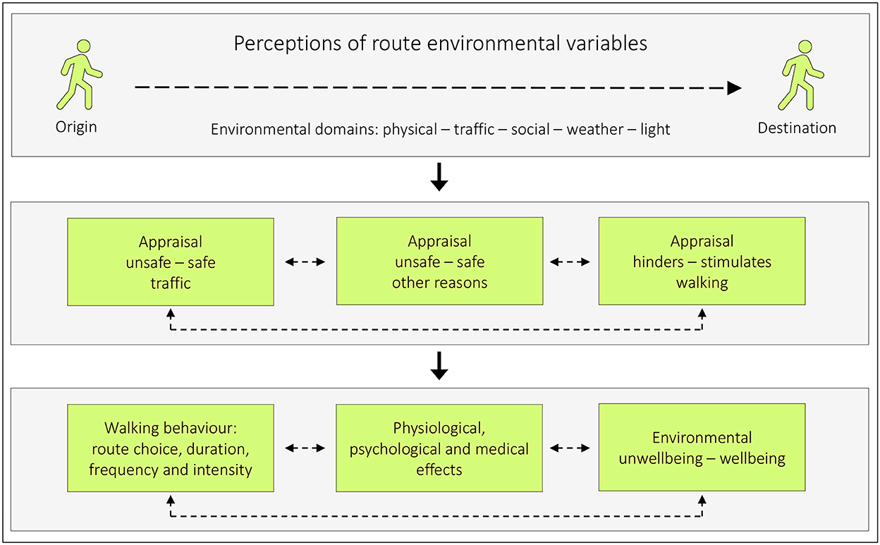
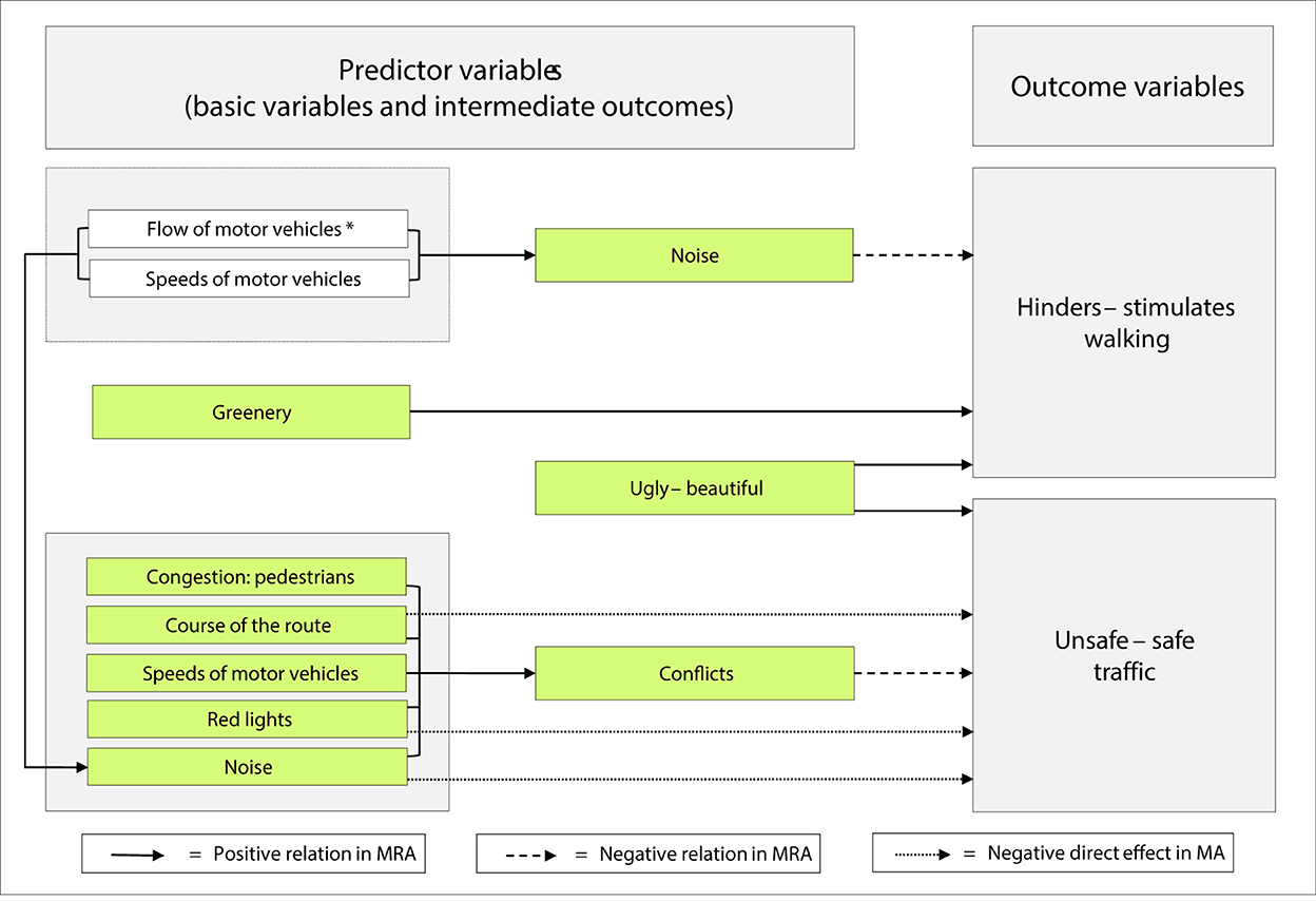
If environmental unwellbeing–well-being is viewed as a final outcome (refer to the conceptual model, Figure 1), at least three intermediate outcomes are constituents of it, namely unsafety–safety for reasons of traffic, ambient conditions that hinder–stimulate walking, and other reasons. Route environmental variables within five different domains can influence these intermediate outcomes and the final outcomes.

Figure 1. A model illustrating how perceptions of route environmental variables may affect pedestrians [modified from (1), p. 150, (7), p. 6]. Route environments consist of different environmental domains: the physical environment (stationary objects such as buildings and trees), the traffic environment (mobile objects such as cars and pedestrians), the social environment (interaction between individuals), weather (wind, rain etc.), and light conditions (natural and artificial). Perceptions of these domains can influence how we appraise unsafety – safety due to traffic, unsafety – safety due to other reasons (such as harassment), and how we appraise the environment with respect to if it is hindering – stimulating for walking. These appraisals can, consecutively, affect our walking behavior (such as route choice and the amount of walking), have physiological, psychological, and medical effects, and will always affect our environmental unwellbeing – wellbeing. The bidirectional hatched lines between the boxes indicate potential mutual relationships.

This conceptual framework is based on experience from long-term educational practice by one of the authors (PS). Further support comes from the scientific literature. Safety (for different reasons) is an important issue among those who walk (3–6). In addition, a need for the supplementary outcome hinders–stimulates walking has been identified [(7), p. 25]. Furthermore, Panter et al. (8) assessed associations between changes in perceptions of the environment en route to work and changes in the level of active commuting. Commuters who reported that it became less pleasant to walk, or perceived more danger while crossing a road, recorded a net decrease in walking. Another example is that traffic volume and speed combined have been described as a barrier to walking affecting hedonic well-being negatively (9). This would in such case refer to the psychological effect in the model. Physical activity can also affect well-being (10), and it is, therefore, important to separate that effect from how walking routes affect environmental unwellbeing–well-being.

Many environmental assessment tools related to walking have been developed. Examples of these include the Neighborhood Environment Walkability Scale (NEWS) by Saelens et al. (11), the Twin Cities Walking Survey (TCWS) by Oakes et al. (12), and the Saint Louis Environment and Physical Activity Instrument by Brownson et al. (13). They all have questions about aspects of the built and traffic environments, using primarily Likert scales of 4-point response.

However, none of them have had the purpose of studying the relations between route environmental variables and the intermediate outcomes unsafety–safety due to traffic or hindering–stimulating for walking (cf. Figure 1). It was therefore considered of great value to develop and evaluate a specialized tool for those purposes: The Active Commuting Route Environment Scale (ACRES) (14, 15). The ACRES is a self-report tool that assesses cycling and pedestrian commuters' perceptions and appraisals of their individual commuting route environments using 15-point response scales.

The aim of this study is to illuminate the role of route environmental variables in relation to the outcomes that hinders–stimulates walking and unsafe–safe traffic, thereby mirroring factors deterring or facilitating walking. Another focus is to explore if there are (i) intermediate outcome variables among the predictors, which represent more basic variables, and (ii) direct or mediating effects between certain variables. We have, therefore, studied male and female commuters (n = 294) rating their own, self-chosen, commuting routes in the inner urban parts of Stockholm, Sweden.

2. Methods 2.1. Procedure and participants

This study is part of a research project entitled Physically Active Commuting in Greater Stockholm (PACS). Active commuters were recruited via two large newspapers in Stockholm (Dagens Nyheter and Svenska Dagbladet) toward the end of May and early June 2004. Inclusion criteria were: (a) being at least 20 years old; (b) living in Stockholm County (excluding the municipality of Norrtälje), and (c) walking and/or cycling the entire distance to one's place of work or study at least once a year. It was emphasized that individuals with all commuting distances were welcome to participate.

The advertisement led to 2,148 volunteers. The first questionnaire, the Physically Active Commuting in Greater Stockholm Questionnaire (PACS Q1), was distributed in September 2004. The response frequency was 94% (n = 2,010). A second questionnaire, the PACS Q2, was distributed in May 2005. The response frequency was 92% (n = 1,819). The participants were cyclists, pedestrians, or dual-mode commuters, that is, those who sometimes cycle and sometimes walk. They commuted in the inner urban or suburban–rural areas of Greater Stockholm, or in both of these areas. For further information about the recruitment process, refer to [(15–17), pp. 65–66].

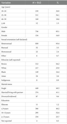
We have exclusively used data on walking commuting from the inner urban area in this study. Some of the participants (26.2%) commuted in the suburban area as well but only their inner urban data have been used. A previous study has shown that cycle commuting in both areas does not affect ratings in either of the areas (15). After cleansing and editing the data, 294 participants (77% women) were included in the analyses: 56.5% were pedestrians and 43.5% were dual-mode commuters. For further descriptive characteristics of the participants, refer to Table 1. The Ethics Committee North of the Karolinska Institute at the Karolinska Hospital approved the study (Dnr 03-637). The participants gave their informed consent.

Table 1. Descriptive characteristics of participants (n = 282–294)*.

2.2. Descriptive characteristics of the participants

Data on sex, age, weight, height, employment, and the number of pedestrian-commuting trips per month were obtained from the PACS Q1. Active commuting trips per year were calculated by adding each of the 12 months' average trip frequency per week, dividing by 12, and multiplying by 52. Educational levels, income, ethnicity, having a driver's license, having access to a car, time leaving home to walk to work, and overall physical and mental health were obtained from the PACS Q2, refer to Table 1.

2.3. The physically active commuting in Greater Stockholm questionnaire (PACS Q1 and Q2)

The PACS Q1 and PACS Q2 are self-report questionnaires in Swedish, which include questions about background factors and different aspects of active commuting. They consist of 35 and 68 items, respectively. The ACRES is included in the PACS Q2. PACS Q1 and Q2, translated into English, can be found as supporting information here (18).

2.3.1. The active commuting route environment scale (ACRES)

To explore relationships between individuals actively transporting themselves between home and work and the route environment, the ACRES was developed and evaluated (14, 15). The pedestrian version of the scale consists of 13 items, refer to Table 2. Two of these items, hinders–stimulates walking and unsafe–safe traffic, are outcome variables but can, in relation to each other and the other items, also act as predictor variables.

Table 2. The Active Commuting Route Environment Scale (ACRES) for pedestrians.

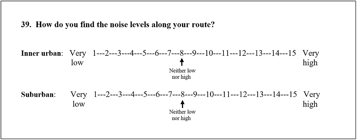
Each item in the ACRES considers the inner urban area of Stockholm, Sweden, and the suburban areas surrounding it within Stockholm County, separately. For an example of an item, refer to Figure 2. The pedestrians were instructed to recall and rate their overall experience of their self-chosen route environments based on their active commuting to their place of work or study during the previous 2 weeks. A more detailed description of the development of the scale, as well as of its validity and reliability for cyclists, has been reported elsewhere (14, 15). In brief, the ACRES was characterized by considerable criterion-related validity and reasonable test–retest reproducibility.

Figure 2. The respondent is asked to encircle the figure that matches the experience, and distinguish the experience in the inner urban area, from the experience in the suburban area. The 15-point response scales, with adjective opposites, have numbered continuous lines, i.e., whole numbers from 1 to 15. In addition, number 8, a neutral option, is labeled, for example, neither low nor high. This is a translation of the original question in Swedish.

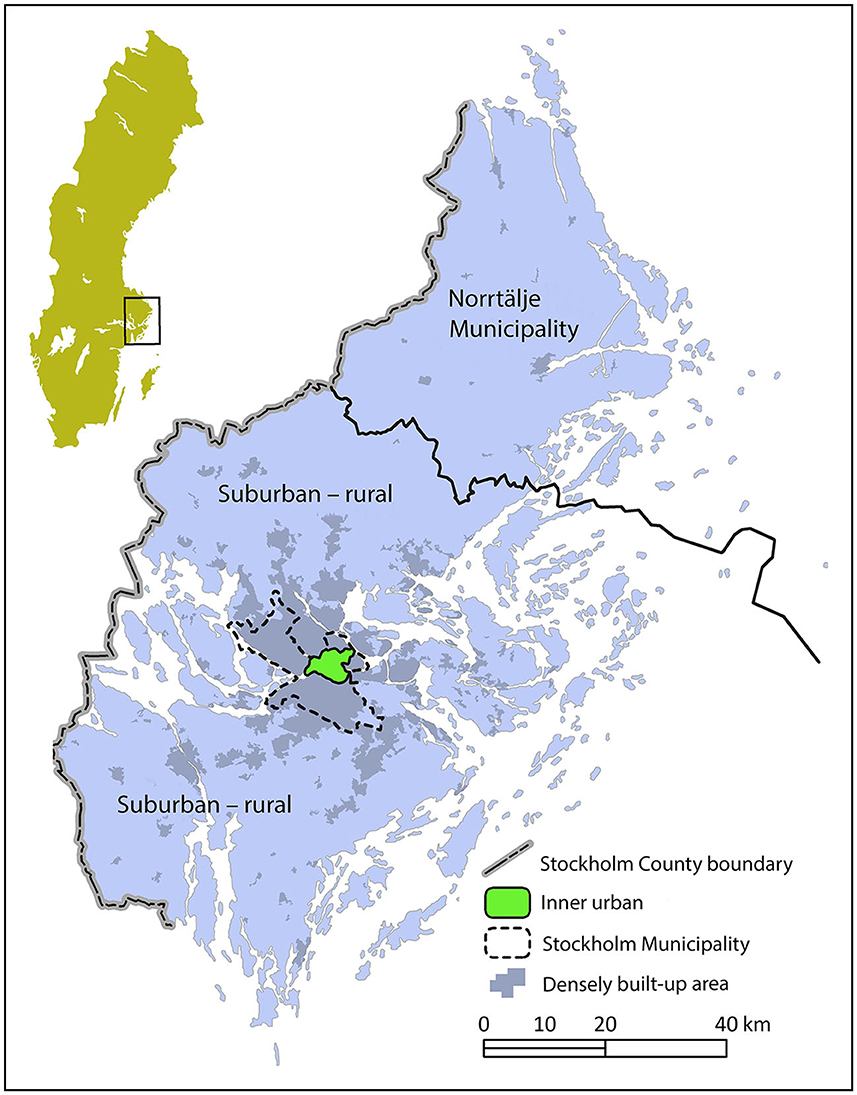
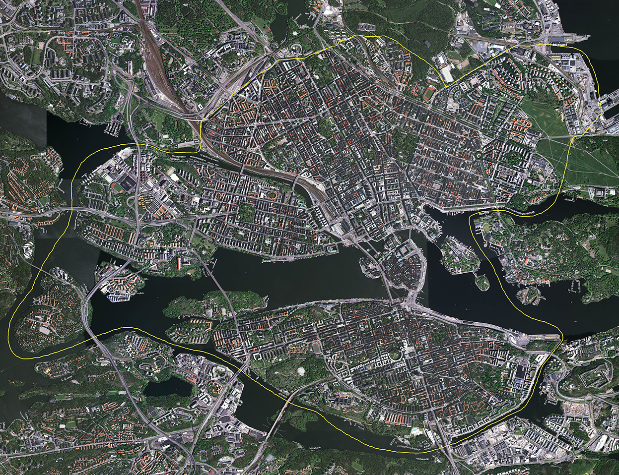
2.4. Study area

The commuting route environments are located in the inner urban area of Stockholm, the capital of Sweden, in the center of a metropolitan area with, at the time, 1.9 million inhabitants (see Figure 3). The inner urban area, in our geographical division of the city, includes the city sections of Gamla stan, Södermalm, Kungsholmen, Vasastan, Norrmalm, and Östermalm. The inner urban area, with blocks organized in grid-like streetscapes (Figure 4), constitutes a different environment compared to the suburban and rural parts of Stockholm County. A more detailed description of the study area can be found in Wahlgren [(19), pp. 62–63].

Figure 3. Map over Sweden and the Stockholm County, with the inner urban study area of the Municipality of Stockholm in green. The markings for the densely built-up areas illuminate the conditions in 2010. North is at the top of the image.

Figure 4. Aerial view of the inner urban study area of Stockholm in 2005. North is at the top of the image (Copyright: Lantmäteriverket, Gävle, Sweden, 2011; Permission 81055230).

2.5. Statistical analyses

Questionnaire data were entered in the Statistical Package for the Social Sciences and analyzed in version 27.0 (IBM SPSS Inc., Somers, NY, USA). All data from PACS Q2, which includes ACRES, were checked for accuracy. Some participants were excluded, mainly because of incorrect or incomplete ACRES data. Participants with no missing ACRES values and no missing values regarding the four descriptive characteristics were used for the analyses. The used descriptive characteristics were sex (dichotomous categorical variable: females = 0 and males = 1), age (continuous variable), education (categorical variable coded as dichotomous: educated at university level = 0 and not educated at university level = 1), and income (categorical variable coded as three categories: ≤ 25,000 SEK/month = 1, 25,001–30,000 SEK/month = 2 and ≥30,001 SEK/month = 3; SEK = Swedish crowns/kronor, year 2005: €1 ≈ 9 SEK; US$1 ≈ 8 SEK) (see Table 1).

Differences between ratings of ACRES between male and female participants were examined with independent t-tests. Correlations between the ratings of the 13 items in the ACRES were assessed using Pearson's correlation coefficient (r). Multiple regression analysis (MRA) was chosen to explore the relationships between the predictor variables and the outcome variables. The background variables sex, age, education, and income were included in the MRA.

Six MRA were run (Models 1–6); Models 1 and 2 had hinders–stimulates walking as an outcome and the items in the ACRES as predictors (Model 1 excluded unsafe–safe traffic and Model 2 included unsafe–safe traffic). The reason for including unsafe–safe traffic as a predictor, a variable that normally acts as an outcome variable, is its possible association with the outcome variable hinders–stimulates walking. Model 1 can be found in the Results section and Model 2 can be found in Supplementary Table A1. Models 3 and 4 had unsafe–safe traffic as an outcome and the items in the ACRES as predictors (Model 3 excluded hinders–stimulates walking and Model 4 included hinders–stimulates walking). The reason for including hinders–stimulates walking as a predictor, a variable that normally acts as an outcome variable is its possible association with the outcome variable unsafe–safe traffic. Model 3 can be found in the Results section and Model 4 can be found in Supplementary Table A2. Model 5 explores conflicts and their relations to relevant items in the ACRES. Model 6 explores the relation between aesthetics (variable name: ugly–beautiful) and all other items in the scale except the two outcome variables.

Five mediation analyses (MA) using PROCESS, a macro designed for SPSS, were run to have a closer look at the impact of one of the intermediate outcomes. PROCESS, written by Professor Andrew F. Hayes, can be downloaded to SPSS from www.processmacro.org (20). To test the indirect effect, we used 5,000 bootstrap samples to generate a confidence interval.

The linearity between the environmental variables (the items in the ACRES) was assessed visually by means of boxplots, error bars and scatterplots. All environmental variables showed reasonable linearity and were therefore used in the analyses. Furthermore, the distribution of the variables was approximately normal according to visual analyses of the boxplots, error bars and scatterplots.

Correlation analyses between the environmental variables were assessed with Pearson's correlation coefficient. The correlations were, in absolute values, r ≤ 0.774 (correlations between the background variable age and the predictor variables were, in absolute values, r ≤ -0.137). According to Tabachnik and Fidell, multicollinearity can be a problem with correlations > 0.90 [(21), pp. 88–90], and according to Field, an approximate method for identifying multicollinearity, that will miss subtler forms, is to pay attention to predictors that correlate very highly, values of r above 0.80 or 0.90 [(22), p. 402].

Due to a previous study (23), where noise protruded as the dominant negative predictor variable among the four variables related to motorized traffic in the ACRES, we have chosen to include noise as a proxy in relation to hinders–stimulates walking. With respect to our other outcomes, unsafe–safe traffic, noise, and speeds of motor vehicles will, due to the same rationale, act as proxies for that quartet of variables.

Our explorative approach included, as stated above, a search for intermediate outcomes among the predictors in this study. This led to an MRA with conflicts as an outcome and relevant items in the ACRES as predictors (Model 5). For this purpose, we analyzed all four traffic variables as predictors (not shown). It resulted in choosing noise and speeds of motor vehicles as proxies for the quartet of traffic variables in relation to conflicts as the outcome. Thereafter, we also included the following predictors: noise, speeds of motor vehicles, congestion: pedestrians, course of the route, and red lights in an MRA with conflicts as the outcome.

Since ugly–beautiful, the aesthetical item, was the only predictor that had a relation with both of our main outcomes, it prompted us to explore what it represents. An MRA, with the items from the ACRES as predictors (excluding the two outcome variables), and with ugly–beautiful as the outcome, was therefore performed (Model 6).

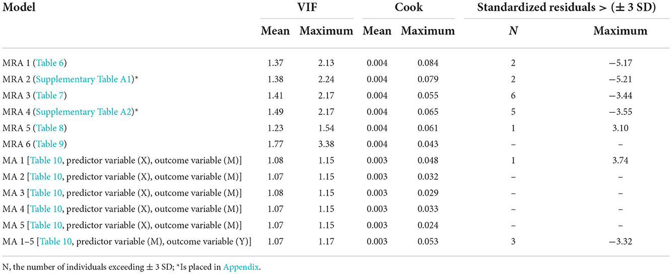
The variance inflation factor (VIF) was used to check multicollinearity. All models with predictor and outcome variables (and the four background variables) were checked (all values ≤ 3.38, mean: 1.26) and indicated no problem [(22), p. 402]. Possible extreme data cases were identified using Cook's distance. No extreme data cases were found in either of the models (all values ≤ 0.084, mean: 0.004), indicating no problem [(22), p. 383].

The top limit for the inclusion of standardized residuals in the models was set to ± 3 SD. A total of 20 individual cases in twelve models had a standardized residual of more than ± 3. They were, however, included in the simultaneous multiple regression analyses since they were few, and had standardized residuals relatively close to the limit for inclusion, as well as no problems with the Cook's distance. A table with the VIF, the Cook's distance, and the standardized residuals can be found in Table 3.

Table 3. The VIF, Cook's distance and standardized residuals.

The values from the MRA are presented as y-intercepts, regression coefficients [unstandardized B, their 95% confidence intervals (CI), and standardized B], as well as adjusted R square (Adj. R2) for the overall models. To indicate significance, a statistical level corresponding to at least p < 0.05 was used. The values from the MA are presented as the standardized total effect, standardized direct effect, and standardized indirect effect of X on Y.

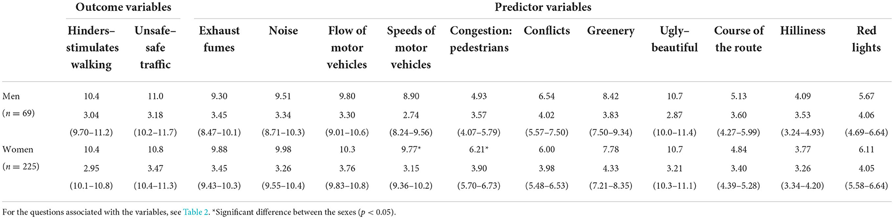
3. Results 3.1. Perceptions of the environmental variables in male and female participants

Levels of the predictor variables and the outcome variables are given in Table 4. In the gender comparisons, significant differences were noted in speeds of motor vehicles and congestion: pedestrians.

Table 4. Levels of perceptions and appraisals of the environmental variables in male and female participants (mean, SD, and 95% CI).

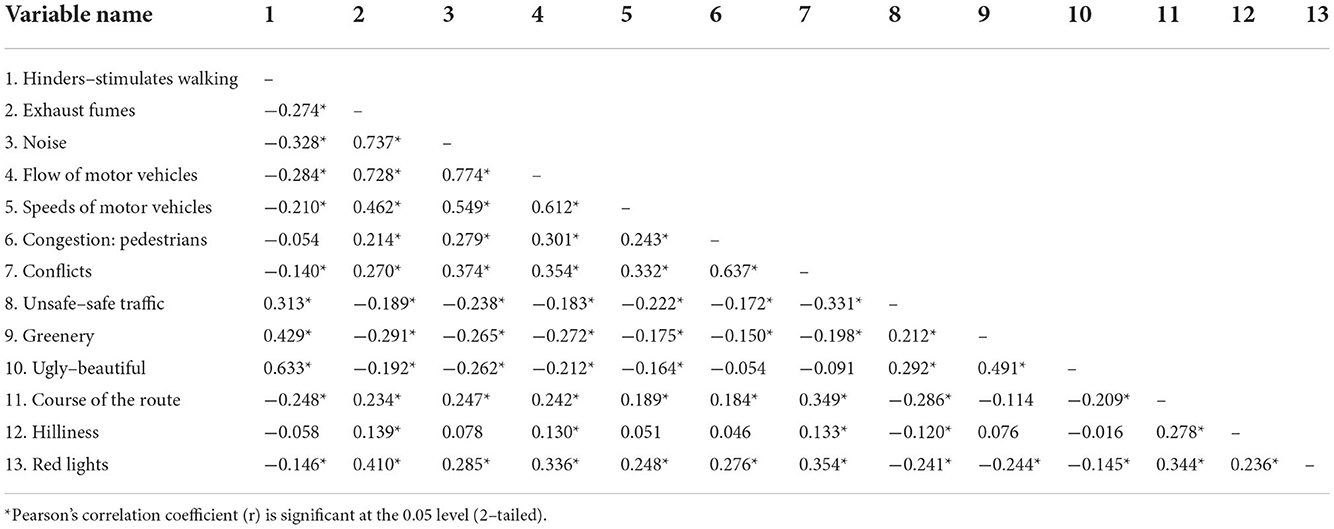
3.2. Correlations between the environmental variables

Correlations between the environmental variables are shown in Table 5. The two highest correlations were between noise and flow of motor vehicles (r = 0.774) followed by between noise and exhaust fumes (r = 0.737). With respect to the outcome variable hinders–stimulates walking, the two highest correlations were with ugly–beautiful (r = 0.633) followed by greenery (r = 0.429). With respect to the other outcome variable unsafe–safe traffic, the two highest correlations were with conflicts (r = −0.331) followed by hinders–stimulates walking (r = 0.313).

Table 5. Correlation matrix for the environmental variables (r).

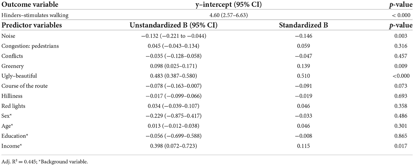
3.3. Relations between the predictor variables and the outcome hinders–stimulates walking

The results of Model 1 (in which the item unsafe–safe traffic was excluded as a predictor) are shown in Table 6. About 45% of the variance of the outcome variable, hinders–stimulates walking, was explained by the predictors in the model (Adj. R2 = 0.445). The regression equation was: Y = 4.60 + 0.510 ugly–beautiful + 0.139 greenery + 0.115 income – 0.146 noise (all p-values ≤ 0.017). Model 2, in which the item unsafe–safe traffic was included as a predictor, is presented in Supplementary Table A1.

Table 6. Model 1; MRA of predictor variables in the ACRES, with hinders–stimulates walking as an outcome, and unsafe–safe traffic excluded.

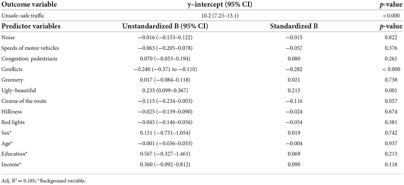
3.4. Relations between the predictor variables and the outcome unsafe–safe traffic

The results of Model 3 (in which the item hinders–stimulates walking was excluded as a predictor) are shown in Table 7. About 20% of the variance of the outcome variable, unsafe–safe traffic, was explained by the predictors in the model (Adj. R2 = 0.185). The regression equation was: Y = 10.2 + 0.215 ugly–beautiful − 0.282 conflicts (all p-values ≤ 0.001). Model 4, in which the item hinders–stimulates walking was included as a predictor, is presented in Supplementary Table A2.

Table 7. Model 3; MRA of predictor variables in the ACRES, with unsafe–safe traffic as an outcome and hinders–stimulates walking excluded.

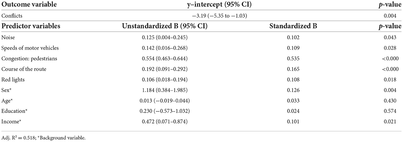
3.5. Relations between conflicts as an intermediate outcome in relation to relevant predictors

The result of Model 5, in which conflicts was the outcome, is shown in Table 8. About 52% of the variance of the outcome variable is explained by the predictors in the model (Adj. R2 = 0.518). The regression equation was: Y = −3.19 + 0.535 congestion: pedestrians + 0.165 course of the route + 0.126 sex + 0.109 speeds of motor vehicles + 0.108 red lights + 0.102 noise + 0.101 income (all p-values ≤ 0.043).

Table 8. Model 5; MRA with conflicts as an intermediate outcome in relation to relevant predictors.

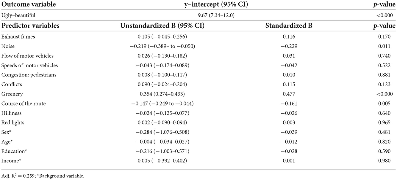
3.6. Relations between ugly–beautiful and other items in the ACRES as predictors

The result of Model 6, in which ugly–beautiful was the outcome, is shown in Table 9. About 26% of the variance of the outcome variable is explained by the predictors in the model (Adj. R2 = 0.259). The regression equation was: Y = 9.67 + 0.354 greenery − 0.219 noise − 0.147 course of the route (all p-values ≤ 0.011).

Table 9. Model 6; MRA with ugly–beautiful as an outcome in relation to other items in the ACRES as predictors.

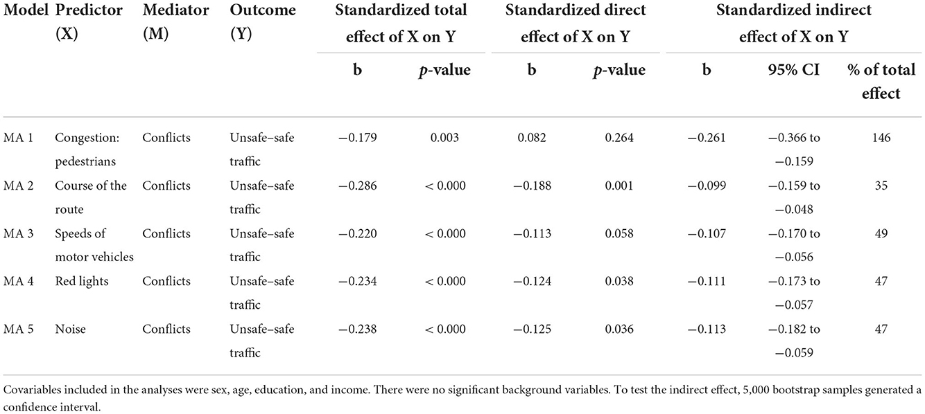
3.7. Mediation

Mediation analyses were run with congestion: pedestrians, course of the route, speeds of motor vehicles, red lights, and noise as predictors and unsafe–safe traffic as an outcome, and conflicts, as a mediator (Table 10). The indirect effect of X on Y was significant in all models and the direct effect was significant in three models.

Table 10. Mediation analyses between predictor variables and unsafe–safe traffic as an outcome with conflicts as a mediator.

4. Discussion

This is probably the first study of the relations between pedestrians' perceptions of route environmental predictors and appraisals of two outcomes of their urban commuting route environments: hinders–stimulates walking and unsafe–safe traffic.

Our main results indicate that ugly–beautiful, the aesthetical item, and greenery appear to strongly stimulate walking, whereas noise hinders it. Notably, the standardized Beta coefficients of ugly–beautiful and greenery add up to 0.65. Furthermore, the aesthetical item is positively related to unsafe–safe traffic, whereas conflicts has the opposite role. Conflicts protrude as the intermediate outcome, representing several basic variables (refer to Figure 5). The mediation analyses demonstrated that some of them also had a direct negative relation with unsafe–safe traffic.

Figure 5. A summary of direct and indirect relations based on commuting pedestrians' perceptions and appraisals of their route environments. In a previous study (23), we have shown that perceptions of both flow and speeds of motor vehicles are related to noise, see * at the box in the upper left corner. MRA = multiple regression analysis; MA = mediation analysis.

4.1. The overall models

About 45% of the variance of the outcome variable hinders–stimulates walking was explained by the environmental predictors in Model 1 (Table 6) and Model 2 (Supplementary Table A1). About 20% of the variance of the outcome variable unsafe–safe traffic was explained by the predictors in Model 3 (Table 7) and Model 4 (Supplementary Table A2). Some of the unexplained variances could be due to missing factors of importance in the ACRES, for example, sidewalks and crosswalks as predictors. Another part of the unexplained variance may be due to the level of reproducibility of the scale (14). In Appendix, comparisons between Model 1 (Table 6) and Model 2 (Supplementary Table A1) as well as between Model 3 (Table 7) and Model 4 (Supplementary Table A2) are commented upon.

In Model 5 (Table 8), where conflicts was the outcome, about 52% of the variance of the outcome variable was explained by the predictors. In Model 6 (Table 9), with ugly–beautiful as the outcome, about 26% of the variance of the outcome variables was explained by the predictors.

4.2. Greenery

Perceptions of greenery are positively related to stimulating walking. This is in line with Wahlgren and Schantz (16) who studied commuting cyclists in the same geographical setting. How can this be comprehended? To begin with, humans have a strong preference for natural versus synthetic environments [(24), p. 67; (25, 26)]. Some theories, for example, Biophilia, suggest that these preferences arise from early humans evolving in natural environments (27).

Second, exposure to natural settings can reduce stress and anxiety, improve mood, mental health, and psychological functioning (28–30). Walking in an environment with greenery has also been reported to improve well-being during the commute (31).

A third possible explanation is that a green environment may lower the rated perceived exertion during physical activity. This has, at least, been shown when running outdoors in a green and blue environment, compared to on a treadmill in a laboratory setting (32); [cf. (33), pp. 125–126]. The authors hypothesized that outdoor environmental cues “masked” the exertion signals outdoors.

4.3. Ugly–beautiful

The aesthetical item is strongly and positively related to hinders–stimulates walking. This is in line with Wahlgren and Schantz (16), who studied commuting cyclists in the same geographical setting. In this study, we also noted that the aesthetical item was positively related to unsafe–safe traffic.

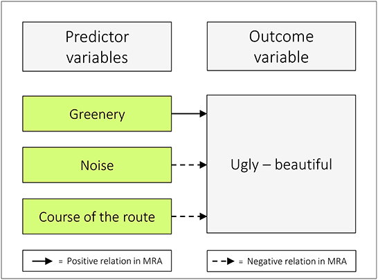
Given that the variable ugly–beautiful influences both of our outcome variables, it is important to thoroughly study the role of this component among those who walk. The fact that the standardized B was 0.51 in relation to hindering–stimulating walking illustrates that the influence of the aesthetical item, in itself, is very strong. This raises the intricate question of what the esthetic item really represents. Our separate analysis, among the predictors in ACRES, revealed that greenery is positively related to ugly–beautiful, whereas noise and the course of the route have opposite roles (refer to Table 9, Figure 6).

Figure 6. Greenery is positively related to ugly – beautiful, whereas noise and course of the route have the opposite role. MRA = multiple regression analysis.

Interestingly, noise impacted the aesthetic item negatively. This is in line with research that has shown that auditory stress, such as aircraft noise and human voices, can affect the perceived aesthetic quality of landscapes (34, 35).

In line with our results, the aesthetic preference seems to be amplified by greenery, such as trees and flowers (36–40).

Spontaneously, it might seem rather odd that a beautiful environment influences perceptions of safety. However, also other studies indicate that an attractive environment may contribute to a feeling of safety (41, 42). According to Drottenborg [(43), p. 19], it is likely that drivers display lower speed in beautiful compared to in ugly traffic environments. Thus, aesthetically rewarding traffic environments seem to be beneficial for traffic safety, which in such case could be an explanation.

In some studies, aesthetics has not been associated with walking for transport (44). In contrast, and in line with our results, aesthetics has been reported to be important for transport walking (4). Since the aesthetical item is related to both of our outcome variables, this variable deserves more scientific attention and should be analyzed from different perspectives, in different settings, and among different populations. This is probably a challenge since aesthetic preferences may vary between individuals (45).

4.4. Noise

In the present study, perceptions of noise were negatively related to hinders–stimulates walking. How can this be understood? First of all, noise can reach almost everyone in the urban streetscape, regardless of different barriers provided by vehicles, vegetation, or other materials. The World Health Organization (WHO) recommends that noise from road traffic should not exceed 53 dB Lden, since, above this level, it is associated with negative health effects [(46), p. 30]. In Stockholm County, 30% of the adult population is exposed to noise levels from road traffic exceeding that level at the façade of their dwelling [(47), p. 15].

In line with what our results indicate, long-term transportation noise annoyance can decrease levels of physical activity (48). Proximity to major roads has also been associated with lower levels of physical activity, independently of noise annoyance (48), and it can possibly be due to a barrier effect of traffic, as has been shown in the case of when major roads are located between residential and green areas (49).

The “noise-problem” can only be partially solved with electric cars. There seems to be a threshold at approximately 30 km/h [(50), p. 35, (51), p. 3]. Below this speed an electric car makes less noise than a conventional car (with an internal combustion engine). For speeds above 30 km/h the friction of the tires is the major source of the noise. In urban areas, where the speed often is above 30 km/h [see e.g., (23)] a transformation of the car fleet toward relatively more electric cars, will most likely not have a pivotal influence on the traffic noise.

Furthermore, with respect to road safety, speed management should be a key issue. In accordance with that, a WHO campaign has been launched to limit the speed in urban areas to 30 km/h [(52), p. 60]. This is in line with the present results that noise and speeds of motor vehicles are negatively related to unsafe–safe traffic.

4.5. Conflicts—An intermediate outcome

Perceptions of conflicts, i.e. the relationships between road users, were negatively related to unsafe–safe traffic. As a matter of fact, conflicts was the only predictor that was negatively related to unsafe–safe traffic in the overall model. Therefore, an MRA with conflicts as the outcome and items in the ACRES that were considered to be relevant were chosen as predictors: noise, speeds of motor vehicles, congestion: pedestrians, course of the route, and red lights (Table 8). The MRA disclosed that all these predictors were positively related to the outcome, that is, all of them are contributing to the perception of conflicts. The two predictors that contributed most strongly (congestion: pedestrians and course of the route) deserve further comments.

Congestion: Pedestrians are strongly and positively related to conflicts, and this is in line with a study by Van Cauwenberg et al. (4), where places that were crowded were disliked by pedestrians. The inclusion of the item course of the route in the ACRES evolved from theories of space syntax (14, 16). The course of the route was measured by the question: “To what extent do you feel that your walking trip is made more difficult by the course of the route? For example, a course with many sharp turns, detours, changes in direction, side changeovers, etc.” These characteristics can be recurrently challenging in terms of new encounters with other street users, and novel traffic situations that can lead to conflicts. Interestingly, the MA (Table 10) disclosed a negative direct effect between the course of the route, red lights, and noise as predictors and unsafe–safe traffic as an outcome.

Thus, we can conclude that conflicts is an intermediate outcome representing several other items in the ACRES.

4.6. Strengths and limitations

This study has both strengths and limitations. To begin with, we have studied pedestrian commuters in their route environments. Normally, active commuting is a highly repetitive behavior along a specific route (53). The commuters are, therefore, very familiar with their route environments and can therefore be viewed as “experts.”

Data were collected using ACRES, an instrument that is characterized by considerable criterion-related validity and reasonable test–retest reproducibility (14, 15). The mean of the intraclass correlation coefficient (ICC) regarding the 18 items for cyclists was 0.65 (0.42–0.87). A major advantage of this scale is that it considers the entire route, from home to the workplace. Researchers have emphasized the importance of taking the entire route into consideration when analyzing walking behavior (54, 55). Furthermore, the research was conducted in the inner urban area of Stockholm, Sweden, where pedestrian commuting is a socially accepted behavior. This increases our chances of a diverse study population, although active commuters represent a limited part of the total population.

Another strength is that this study is based on subjective measures of perceptions and appraisals. This is valuable since it is known that a given objective measure can, dependent on individuals' sensitivity, be rated differently. For example, an objective level of noise in dB can induce quite diverse sensations among individuals (56).

With reference to limitations, the advertisement recruitment strategy of the participants could possibly increase the risk of self-selection bias, for example, not everyone is reading newspapers. However, this sampling method has been compared to street recruitment of cyclists regarding ratings of route environments in the same area (15). It was hypothesized that the street recruitment strategy represented the population with greater certainty than the advertisement strategy. Overall, the participants' ratings indicated a reasonably good correspondence between the two groups (15). Furthermore, the characteristics of the two samples, with respect to background factors such as age, gainful employment, and education, showed relatively good agreement [(17), pp. 65–69]. In addition to that, the present participants were characterized by similar levels of gainful employment and income as the pedestrians in the National Travel Survey, who were randomly recruited [(17), pp. 109–110]. Nevertheless, a consequence of possible selection bias is that the results should be interpreted carefully.

5. Conclusion

Aesthetics and greenery appear to be strong stimulating factors of walking, whereas perceptions of noise, as a proxy for traffic, hinder it. Furthermore, aesthetics is positively related to unsafe–safe traffic, whereas conflicts has the opposite role. Conflicts is an intermediate outcome, representing several predictors. Greenery is positively related to aesthetics whereas noise and the course of the route have the opposite role.

Numerous things can be done to improve the quality of the urban environment. A modal shift from individual car use to active commuting is one such example. If policymakers and urban practitioners can focus on the facilitating variables when designing and developing urban route environments, it could possibly be a game changer with respect to public health, attracting new pedestrians, and simultaneously stimulating those who already walk, to keep on walking.

Data availability statement

The raw data supporting the conclusions of this article will be made available by the authors, without undue reservation.

Ethics statement

The studies involving human participants were reviewed and approved by the Ethics Committee North of the Karolinska Institute at the Karolinska Hospital, Stockholm, Sweden. The patients/participants provided their written informed consent to participate in this study.

Author contributions

Conceptualization, supervision, project administration, and resources: PS and LW. Funding acquisition: PS. Visualization, writing—review and editing, writing—original draft preparation, and formal analysis: DA, LW, and PS. Data curation and investigation: DA and LW. Methodology: DA and PS. All authors contributed to the article and approved the submitted version.

Funding

This study was supported by the Research Funds of the Swedish Transport Administration (TRV 2017/63917-6522). The funding source had no involvement in any aspect of the study.

Acknowledgments

The authors are grateful to the volunteers for participating in the study and for the technical assistance of Erik Stigell, LW, Golam Sajid, Eva Minten, and Per Brink, as well as PS and Erik Stigell for the development of the ACRES. We also extend our gratitude to Dr. Rui Wang for statistical advice and Dr. Charlotta Eriksson for valuable comments on noise and health. Finally, many thanks to the associate editor and the reviewers for your service and constructive as well as valuable comments.

Conflict of interest

The authors declare that the research was conducted in the absence of any commercial or financial relationships that could be construed as a potential conflict of interest.

Publisher's note

All claims expressed in this article are solely those of the authors and do not necessarily represent those of their affiliated organizations, or those of the publisher, the editors and the reviewers. Any product that may be evaluated in this article, or claim that may be made by its manufacturer, is not guaranteed or endorsed by the publisher.

Supplementary material

The Supplementary Material for this article can be found online at: https://www.frontiersin.org/articles/10.3389/fpubh.2022.1012222/full#supplementary-material

References

1. Schantz P. Physical activity behaviours and environmental well-being in a spatial context. In:Schaerström A, Jörgensen SH, Kistemann T, Sivertun Å, , editors. Geography and Health—A Nordic Outlook. Stockholm: Swedish National Defence College; Trondheim: Norwegian University of Science and Technology (NTNU); Bonn: Universität Bonn (2014). p. 142–56.

Google Scholar

2. World Health Organization. Preamble to the Constitution of the World Health Organization. New York, NY: World Health Organization (1948). 18 p.

Google Scholar

4. Van Cauwenberg J, Van Holle V, Simons D, Deridder R, Clarys P, Goubert L, et al. Environmental factors influencing older adults' walking for transportation: a study using walk-along Interviews. Int J Behav Nutr Phys Act. (2012) 9:85. doi: 10.1186/1479-5868-9-85

PubMed Abstract | CrossRef Full Text | Google Scholar

5. Van Cauwenberg J, Clarys P, De Bourdeaudhuij I, Van Holle V, Verte D, De Witte N, et al. Physical environmental factors related to walking and cycling in older adults: the Belgian aging studies. BMC Public Health. (2012) 12:142. doi: 10.1186/1471-2458-12-142

PubMed Abstract | CrossRef Full Text | Google Scholar

6. Alfonzo MA. To walk or not to walk? The hierarchy of walking needs. Environ Behav. (2005) 37:808–36. doi: 10.1177/0013916504274016