Equipment description

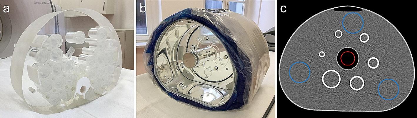
The Spark (Fig. 1) was affixed to the benchtop of a Triumph LabPET4/CT dual-modality system (TriFoil Imaging, Chatsworth, USA), and although the Triumph’s imaging systems were unused in this study, the animal bed was used for positioning radioactive source distributions in SPECT tests. The Spark’s detector housing, detector cover, and collimator were manufactured from tungsten that yield an overall length, width, and height of \(150.4\times 138.1\times 56.4\,\hbox ^\) when assembled. The detector housing accepts an aluminum scintillator housing assembled with a \(102\times 102\times 3\,\hbox ^\) monolithic CsI(Na) scintillation crystal (Saint-Gobain Crystals, Hiram, USA) and a 2 mm-thick glass light guide. Saint-Gobain BC-631 silicone grease was used to optically couple the light guide to a \(14\times 14\) SensL C-series SiPM array comprised of 6 mm sensors with a 7.2 mm pitch on a printed circuit board (ON Semiconductor, Phoenix, USA). The SiPM array operates at room temperature without a cooling system. Further information regarding the construction of the Spark may be obtained from the manufacturer.

Fig. 1

The Cubresa Spark preclinical SPECT scanner and mouse-sized NEMA triple line source scatter phantom illustrated in a photograph of the system (left) and an axial cutaway view of the detector head modelled in GATE (right). The labelled components in the photograph are the Triumph LabPET4/CT (1), Cubresa Spark gantry (2), mouse-sized NEMA triple line source scatter phantom (3), the animal bed (4), and the SPECT detector head (5). The triple line source phantom dimensions are included for scale

As outlined in Table 1, the Spark performance was assessed with two interchangeable tungsten collimators (Scivis GmbH, Göttingen, Germany): a single-pinhole (SPH) collimator for high-resolution planar and tomographic imaging, and a multiplexing multi-pinhole (MPH) collimator for high-resolution tomography with increased sensitivity. The SPH collimator has a non-focusing right-circular double-cone pinhole, and the MPH collimator uses a \(5\times 5\) array of focusing right-circular double-cone pinholes where each row focuses on a different volume of interest (VOI) in the tomographic field of view (FOV) [27]. The area of the detector used for imaging \(\gamma\)- and X-rays has a useful field of view (UFOV) and central field of view (CFOV) of 84.5 mm and 63.375 mm, respectively.

Table 1 Geometric specifications of pinhole collimators

The Spark was delivered with Scivis’ HiSPECT reconstruction software, which was preconfigured solely for the MPH collimator. Precise information regarding the MPH collimator geometry was not readily available, and as a result, this restricted the simulation model to the SPH collimator only. Measured and simulated SPH SPECT images were reconstructed with the Software for Tomographic Image Reconstruction (STIR) v5.1.0 using the pinhole-SPECT acquisition matrix [28,29,30].

Prior to measurement, the SPECT system was calibrated for energy, linearity, uniformity, center of rotation, and aperture-to-detector distance [31, 32]. Radionuclide activity measurements were performed with a Capintec CRC-55tR dose calibrator (Mirion Technologies, Florham Park, USA). Various phantoms and source positioning jigs were fabricated in-house to adhere to the NEMA protocol, and each required device is described in the following sections.

Simulation description

A model of the Spark detector head (Fig. 1) was created using the SPECThead system in the GATE v9.0 Monte Carlo toolkit [10] compiled with Geant4 10.06.p01 [11] and Rapid Object-Oriented Technology (ROOT) 6.14.04 [33]. Simulations were distributed over 12 cores on an HP Z820 workstation operating Ubuntu 18.04.5 LTS with two Intel Xeon E5-2630 2.3 GHz hexa-core CPUs and 64 GB of 1600 MHz DDR3 memory. ROOT output was combined into one file and then converted to Cubresa’s list mode format for further processing.

Complex detector geometry was modelled with standard tessellation language (STL) files provided by Cubresa, and simple geometric volumes such as the scintillator, light guide, SiPM array, printed circuit board, and phantoms were modelled with predefined shapes available in GATE. Material properties were assigned to their respective volumes using the Geant4 and GATE materials database. More specifically, the modelled collimator, detector housing, and detector cover materials were tungsten, the scintillator housing was aluminum, the scintillation crystal was CsI, the light guide was glass, the SiPM array was silicon, and the printed circuit board was epoxy. The scintillation process, optical photon transport, and light detection were not simulated to save computing time. Therefore, the silicone optical grease was negated from the simulation model. Other excluded components were the 3.5 mm-thick carbon fiber animal bed due to its application in only two NEMA tests with minimal attenuation in SPECT acquisitions, and the MPH collimator due to restricted knowledge of the pinhole geometry. For reasons detailed in the Discussion, the SPH collimator was modelled with a 0.85 mm-diameter pinhole to better match the simulated collimator-detector response function to measurement.

Physics processes were initialized with the Geant4 standard electromagnetic physics package option 4 (emstandard_opt4) [11]. Particle production cuts were set at the default value of 1 mm corresponding to a few keV in most materials, except the scintillation crystal and pinhole knife-edge where the threshold was set to 1 keV. Radioactive sources were defined as an isotropic UserSpectrum source of \(\gamma\)-rays with emissions defined from the Table of Radionuclides [34]. The Spark’s electronics, i.e., signal processing chain, were modelled using the following GATE digitizer modules: the adder, readout, energy blurring, spatial blurring, pile-up, dead time, and efficiency. Figure 2 presents the digitizer chain with the values set for parameters of interest. Digitizer parameters were determined empirically from measurement by simulating a range of values for a given digitizer parameter, fitting a cubic spline to the simulated results, then interpolating the digitizer parameter at the measured result. However, the pile-up timing resolution \(t_\text \) was calculated as

$$\begin t_\text = \frac (P_0 + 2P_1)} \end$$

(1)

where \(P_0\) and \(P_1\) are the counts in the primary and first order pile-up peaks, respectively, and \(R_\text \) is the true input count rate [35].

Fig. 2

Digitizer signal processing model of the Spark’s readout electronics used in GATE. Interactions in the scintillation crystal were recorded as hits following Geant4 particle generation and transport through modelled materials. Hits were subsequently filtered through the digitizer modules to obtain singles corresponding to the detected signal after processing by the front-end electronics. Digitizer parameters were determined empirically from measurement by simulating a range of values for a given digitizer parameter, fitting a cubic spline to the simulated results, then interpolating the digitizer parameter at the measured result, except for the pile-up timing resolution which was calculated with Eq. 1

NEMA performance characterization and SPECT model validation

Performance characterization of the Spark was made according to the NEMA NU 1-2018 protocol, with tests briefly described in the following sections. The radionuclide for all tests was technetium-99m (\(^\text \)Tc) except for the Multiple Window Spatial Registration test which used Gallium-67 (\(^\)Ga). An energy window width of 30% was centered on the reference photopeak(s) when generating projection images for all tests. The UFOV and CFOV were defined with electronic masking, and images had 0.1 mm isotropic pixels unless stated otherwise. Measured data were acquired according to total acquisition time or counts through an open energy window. Note that acquired counts refer to the computer’s unprocessed estimate of counts determined from the optical light collected from the scintillation crystal, which Cubresa’s proprietary data processing software then converts to detected/observed counts stored in list mode data in terms of position, energy, and time. Simulations were then configured based on measurements of data acquisition time, radioactivity, radioactive source distribution, and system geometry, except for the SPH collimator pinhole diameter. No corrections were applied to the simulated data at any stage. Validation of the GATE model was based on reporting parameter comparisons between measured and simulated NEMA results.

Tests of intrinsic gamma camera detector characteristicsIntrinsic spatial resolution and linearity

Intrinsic spatial resolution refers to the \(\gamma\)-camera’s ability to localize an ionizing photon’s interaction site within the detector, and intrinsic linearity reflects the distortion of those interaction sites throughout the detector’s FOV. This test was performed with a 2.5 mm-thick tungsten planar mask comprised of a \(3\times 3\) grid of 0.8 mm-wide and 26.5 mm-long parallel slits having adjacent slit centers separated by 31.5 mm, and a Derenzo pattern with  mm-diameter holes. An Eppendorf tube containing a 50 MBq point source was centered 65 cm above the face of the detector, and 15 million counts were acquired. Intrinsic resolution and linearity were assessed from line spread functions (LSFs) and analyzed according to the procedures defined by the NEMA NU 1-2018 protocol. A millimeters-per-pixel calibration factor was also calculated using line profile spacing to convert relevant image dimensions to physical units in relevant NEMA tests.

Normally, the mask-slit geometry would yield the limiting intrinsic spatial resolution. However, due to the spatial resolution performance of the SiPM detector, the mask-slit geometry described above produced LSFs that were wider than the intrinsic spatial resolution. Therefore, a secondary test was performed using a non-NEMA source geometry to extract the limiting resolution. A point spread function (PSF) was created with a pencil beam emitted from a tungsten line source holder with a tunnel 0.4 mm in diameter, 10.0 mm in length, and centered 1.0 mm above the middle of the detector with a 1.0 cm-thick aluminum plate. A total of 100,000 counts were acquired from a 170 MBq line source established in a glass capillary tube (inner diameter \(\varnothing _\text =1.15\,\hbox \), outer diameter \(\varnothing _\text =1.50\,\hbox \), length \(L=75\,\hbox \)) and secured in the line source holder. The PSF was then analyzed following the methods applied to the LSFs produced with the mask-slit geometry.

Intrinsic flood field uniformity

The intrinsic uniformity quantifies the \(\gamma\)-camera’s response to a uniform radiation flux. An 8 MBq point source was centered 65 cm above the face of the detector, and 100 million counts were acquired. The measured and simulated flood field projection images with 1 mm pixels were smoothed once by convolution with the NEMA smoothing filter, and measured data were corrected for uniformity. The integral uniformity was calculated using

$$\begin \text \,(\%) = \frac - \text } + \text } \times 100 \end$$

(2)

where \(\text \) and \(\text \) refer to the maximum and minimum pixel values within the FOV. Similarly, the differential uniformity was calculated with Eq. 2 from the \(\text \) and \(\text \) in a set of five contiguous pixels in a row or column.

Multiple window spatial registration

The multiple window spatial registration (MWSR) test was performed with 11 MBq of \(^\text \)Ga to assess the Spark’s ability to accurately localize photons of different energies when imaged through different energy windows. The previously described pencil beam source holder (see Intrinsic spatial resolution and linearity) was positioned in a 1.0 cm-thick aluminum plate at nine locations along the detector axes, including the middle of the detector, \(0.4\times\), and \(0.8\times\) the distance to the edge of the UFOV. A total of 4 million counts were acquired at each position, and projection images were generated from each photopeak. The maximum axial and transaxial displacements of PSF centroids were then calculated. Overall spatial registration accuracy was also assessed according to the mean Euclidean distance between each centroid and the average centroid location.

Intrinsic count rate performance in air: decaying source method

The count rate performance describes the \(\gamma\)-camera’s ability to process one detection event before moving on to another, and the number of detected counts may be fewer than input events because of dead time and/or pile-up. Two models exist to describe idealized dead time behaviour: paralyzable and non-paralyzable dead time [36]. The Spark’s behaviour is well described with a paralyzable model using the equation

$$\begin \text = \text \,\textrm^\tau } \end$$

(3)

where \(\text \) is the observed count rate, \(\text \) is the input count rate, and \(\tau\) is the system dead time. Furthermore, \(\text \) can be affected by pile-up, which occurs when a true event at time \(t=0\) is followed by subsequent events in the interval \(0<t<\tau\), followed by an event-free interval of length \(\tau\). Using the decaying source method, the dead time was calculated from the intercept and slope of Eq. 4:

$$\begin \lambda t + \ln \text = -\text _0 \tau \textrm^ + \ln \text _ \end$$

(4)

where \(\lambda\) is the decay constant, t is the time, \(\text _0\) is the true input rate at the beginning of measurement, \(e^\) is the abscissa, and \(\lambda t + \ln \text \) is the ordinate [36].

Care was taken to minimize scatter during count rate performance assessment by securing an Eppendorf tube containing 235 MBq in a tungsten Capintec 511 Dose Drawing Syringe Shield. The shield was capped with a lead lid, and a 6.0 mm-thick copper plate covered the open side of the source holder. The source was placed at a distance of \(5\times\) UFOV above the detector face to produce a uniform radiation field. Counts were measured for 60 s and simulated for 10 s in 60 min intervals, and the last data point was acquired when the observed count rate dropped below 600 cps to determine \(\text _0\) accurately. All data were corrected for radioactive decay, and the measured data were corrected for background noise and uniformity. Measured count rate data were utilized to configure the digitizer pile-up, dead time, and efficiency modules in the simulation model. Following the NEMA protocol, the intrinsic count rate performance was analyzed in terms of the maximum \(\text \) and 20% loss \(\text \).

Intrinsic energy resolution

The energy resolution characterizes a radiation detector’s response to a monoenergetic radiation source and describes its ability to distinguish between different energies of that radiation. The formal definition is

$$\begin \text \, (\%) = \frac}} \times 100 \end$$

(5)

where FWHM is the full width at half maximum of the photopeak calculated according to NEMA’s resolution methodology in this context. The Spark’s intrinsic energy resolution was assessed using 0.6 keV bins with the count rate data point immediately below the 20% loss OCR introduced in the previous section (Intrinsic count rate performance in air: decaying source method). This data point satisfies all NEMA conditions while offering count rate traceability. The simulated data point below the 20% loss OCR was re-simulated with a 60 s acquisition time to obtain count statistics comparable to the measurement. Note that a keV-per-channel calibration factor was not calculated with cobalt-57 (\(^\text \)Co) since a vendor-specific energy calibration is automatically applied to list mode data.

Tests of gamma camera detectors with collimators

In this study, system or extrinsic measurements primarily involved the SPH collimator due to its applicability in planar scintigraphy yielding unambiguous projection images. Measurements with the experimental MPH were included where applicable.

System spatial resolution without scatter

The system spatial resolution without scatter represents the \(\gamma\)-camera’s limiting ability to localize a photon interaction site in the detector when combining collimator and intrinsic factors. Acquisitions were performed in the axial and transaxial directions using a precision glass capillary tube (\(\varnothing _\text =0.4\,\hbox \), \(\varnothing _\text =0.8\,\hbox \), \(L=75\,\hbox \)). The capillary tube contained 10 MBq of radioactivity, and 100,000 counts were acquired at positions of  mm from the face of the SPH collimator. NEMA’s resolution methodology was applied to calculate resolution from LSFs. Results were corrected for magnification to compare resolution in the object rather than the detector. A plot of the average system resolution as a function of source-to-collimator distance was generated with a linear least squares fit to characterize the system resolution.

System spatial resolution with scatter

The presence of a scattering medium degrades image quality in terms of projection image blurring, reduced contrast in reconstructed images, and decreased quantitative accuracy [37]. Thus, the system spatial resolution with scatter was assessed with a mouse-sized NEMA triple line source scatter phantom fabricated from an acrylic cylinder (\(\varnothing =25.4\,\hbox , L=60\,\hbox \)) with three 0.8 mm-diameter bores for precision capillary tubes: one at the center and two separated by 90\(^\) with a 10 mm radial offset. One precision capillary tube containing 10 MBq was inserted into the central bore of the scatter phantom, and 100,000 counts were acquired axially and transaxially at capillary tube positions of  mm from the face of the collimator. Analysis of the resulting projection images followed the methods outlined in System spatial resolution without scatter.

System planar sensitivity

The system planar sensitivity characterizes the number of detected counts per unit activity to evaluate a collimator’s count rate performance. A 35.0 mm-diameter petri dish was filled with a solution of 2 ml of water and injected with a calibrated activity of \(A_\text =210\,\text \) for the SPH dataset and \(A_\text =25\,\text \) for the MPH dataset. The internal base of the radioactive solution was placed at source-to-collimator distances of \(D=\\,\hbox \), and 4 million counts were acquired at each position in measurement. In contrast, counts were acquired for 100 s at each position in simulation to save on computing time. Data were acquired from the largest to the smallest distance with activity levels ranging from \(A_\text \) to \(\sim\)15 MBq to minimize pile-up and dead time effects, namely in the SPH acquisition. Measured data were corrected for uniformity, and then, the decay-corrected count rate R was calculated for each acquisition i as

$$\begin R_i = \lambda C_i \textrm^)} \times \big (1-\textrm^,i}}\big )^ \end$$

(6)

where \(C_i\) is the summed counts from the projection image, \(T_i\) is the acquisition start time, \(T_,i}\) is the acquisition duration, and \(T_\text \) is the time of activity calibration. Using a standard Levenberg–Marquardt nonlinear least squares fit technique, the decay-corrected count rate and source-to-collimator distance for each SPH acquisition were fit with the function

$$\begin R_i = c_0 + c_1 \textrm^ \end$$

(7)

where \(c_0\), \(c_1\), and \(c_2\) are fitting parameters. The total system sensitivity \(S_\text \) was then calculated as

$$\begin S_,i} = \frac} \end$$

(8)

and plotted against the source-to-collimator distance to characterize the sensitivity. Note that NEMA’s protocol utilizes fit parameters from Eq. 7 to compute a collimator penetration factor for detected counts in a given region of interest (ROI). This analysis was excluded as it does not apply to pinhole collimators. Furthermore, Eq. 7 does not apply to the MPH collimator due to the focusing orientation of pinholes.

Tests specific to tomographic camera systems

SPECT projection data were acquired from \(0^\) to \(270^\) in a \(208\times 208\) matrix with 0.5 mm isotropic pixels and then reconstructed with nine iterations of the maximum likelihood expectation maximization (MLEM) algorithm in 0.25 mm isotropic voxels. SPH SPECT data were acquired in \(3^\) increments and then reconstructed with STIR in a \(230\times 184\times 184\) matrix, and MPH SPECT data were acquired in \(90^\) increments and then reconstructed with HiSPECT in an \(80\times 144\times 144\) matrix. HiSPECT software only supports the MLEM algorithm, whereas STIR’s pinhole-SPECT software permits access to STIR’s extensive library of algorithms and corrections for the spatially variant collimator-detector response and attenuation. Thus, SPH SPECT data were also reconstructed with the filtered back projection (FBP) algorithm using a ramp filter to adhere to the NEMA protocol.

SPECT reconstructed spatial resolution without scatter

The reconstructed spatial resolution without scatter reflects the limiting size of a radioactive distribution that can be observed with the \(\gamma\)-camera. Three point sources in air were established in precision capillary tubes with a mean activity of \(0.274\pm 0.007\) MBq and an axial extent of \(\sim\)0.4 mm. To conform to the small reconstructed FOV of the MPH collimator (see Table 1), one point source was centered on the axis of rotation, and the two remaining point sources were positioned at ± 75% of the distance to the edge of the FOV, i.e., ± 5.25 mm axially and ± 11.25 mm transaxially. The point sources were set in place, and 300,000 counts were acquired across all projections in the SPH and MPH acquisitions to directly compare tomographic resolution. Cubic ROIs were centered around each reconstructed point source and summed along each axis to calculate the radial, tangential, and axial resolution without scatter according to the NEMA protocol.

SPECT reconstructed spatial resolution with scatter

The reconstructed spatial resolution with scatter was assessed with the mouse-sized NEMA triple line source scatter phantom described in System spatial resolution with scatter. Three capillary tubes containing a mean activity of \(9.4\pm 0.1\) MBq were inserted into the phantom and centered axially in the FOV with peripheral line sources placed at \(0^\) and \(270^\) to maximize the amount of scatter contributing to projection images over the extent of rotation. The line sources in the scatter phantom were set in place, and 5 million counts were acquired across all projections in the SPH and MPH acquisitions to directly compare tomographic resolution. The reconstructed images were summed axially to obtain three 3.5 mm-thick transverse slices: one at the center of the FOV and two at ± 75% the distance to the edge of the respective axial FOV. A square ROI was centered on each resulting PSF to calculate the central, radial, and tangential resolution with scatter according to the NEMA protocol.

SPECT volume sensitivity, uniformity, and variability

The system volume sensitivity (SVS) reports the total system sensitivity to a uniform activity concentration in a cylindrical phantom. An acrylic phantom (\(\varnothing _\text =26\,\hbox \), \(\varnothing _}=28\,\hbox \), \(L_\text =21\,\hbox \)) was filled with water containing 1.75 MBq/ml then centered along the axis of rotation in the \(\gamma\)-camera’s image space. The phantom was set in place, and SPH and MPH SPECT acquisitions were obtained with 10 s and 60 s projections, respectively. The measured data were corrected for uniformity, then the SVS was calculated as

$$\begin \text = \frac} \end$$

(9)

where A is the average count rate (total detected counts divided by total elapsed time including time for rotation) and \(B_\text \) is the activity concentration halfway through the acquisition. By normalizing the \(\text \) by the axial extent L of the cylindrical phantom in the reconstructed image, the volume sensitivity per axial centimeter (\(\text \)) was calculated as

$$\begin \text = \frac}. \end$$

(10)

The \(\text \) was then multiplied by the reconstructed axial FOV of the collimator to obtain a useful approximation of the total system response to a broad distribution of radioactivity.

Although it is not a defined NEMA test, the volume uniformity was evaluated from images of the cylindrical phantom reconstructed with the MLEM algorithm. Integral uniformity was calculated with Eq. 2 from a VOI covering 75% of the phantom’s imaged length and 60% of the phantom’s inner diameter. Within this VOI, the variability was determined from the coefficient of variation (CV):

$$\begin \text \,(\%) = \frac \times 100 \end$$

(11)

where \(\sigma\) is the standard deviation and \(\mu\) is the mean voxel value within the VOI.