1. Introduction

The proportion of older adults or elderly is increasing across the world. Globally, the number of adults aged 65 years or above surpassed the number of children under the age of 5 for the first time in 2018. Further, the share of the global population aged 65 years or above is projected to rise from 10% in 2022 to 16% in 2050 (Ritchie and Roser, 2019; United Nations Department of Economic and Social Affairs, Population Division, 2022). This upward shift in the age distribution of the global population makes it crucial (Cabeza et al., 2016) to identify the neuronal correlates of age-related decline in cognition, perception and motor performance. The advent of cutting-edge neuroimaging technologies has facilitated the study of anatomical and functional changes in the human brain during the healthy aging process (Grady, 2012; Tromp et al., 2015). Specifically, studies employing functional magnetic resonance imaging (fMRI) methods (Spreng et al., 2010; Eyler et al., 2011; Rodriguez-Sabate et al., 2022) have shed light on the altered activity of brain regions that are necessary for optimal cognitive performance in elderly individuals, including the prefrontal, medial temporal and parietal cortices (Nyberg et al., 2010; Grady, 2012; Addis et al., 2015). There is also an increasing interest in the development of novel intervention strategies for reversing the effects of age-related functional decline. Non-invasive brain stimulation techniques such as transcranial direct current stimulation (tDCS), transcranial alternating current stimulation (tACS), and transcranial magnetic stimulation (TMS) offer an attractive option to modulate neuronal plasticity and improve learning processes in older individuals (Nitsche et al., 2008; Reis et al., 2009; Zimerman and Hummel, 2010). Neuroimaging techniques such as fMRI can not only record the activity of individual regions in the human brain, but also capture the correlations between the activities of these brain regions (Logothetis, 2008), thereby revealing the underlying functional connectivity networks (FCNs). Numerous efforts have been undertaken to characterize age-related changes in FCNs using concepts and tools from network science and graph theory (Bassett and Sporns, 2017). Remarkably, graph-theoretic studies on resting-state fMRI (rs-fMRI) datasets of healthy young and healthy older individuals have demonstrated age-related changes in several network-based measures including clustering coefficient, shortest path length, global efficiency, local efficiency, and modularity (Achard and Bullmore, 2007; Sala-Llonch et al., 2014; Song et al., 2014; Geerligs et al., 2015; Li et al., 2016). Recent graph-theoretic studies have combined data from diffusion tensor imaging (DTI) and rs-fMRI scans of healthy aging participants in the Max Planck Institute Leipzig Study for Mind-Body-Emotion Interactions (MPI-LEMON) (Babayan et al., 2019) to analyze the influence of white matter hyperintensities (WMH) and global fractional anisotropy (gFA) on resting-state FCNs (Porcu et al., 2020, 2021).

In recent years, several geometric notions of discrete Ricci curvature (Forman, 2003; Ollivier, 2007; Sreejith et al., 2016; Samal et al., 2018) have been introduced as novel tools for the analysis of complex networks (Bianconi and Rahmede, 2017; Boguñá et al., 2021). Discrete Ricci curvatures allow for a rigorous characterization of network structure by accounting for higher-order correlations in a network (Kartun-Giles and Bianconi, 2019), and have found important applications such as community detection in networks (Ni et al., 2019; Sia et al., 2019; Tian et al., 2022) and indicators of critical events in financial markets (Sandhu et al., 2016; Samal et al., 2021). Forman-Ricci curvature (FRC) (Forman, 2003; Sreejith et al., 2016) and Ollivier-Ricci curvature (ORC) (Ollivier, 2007) are the two commonly-used notions of discrete Ricci curvature for analysis of complex real-world networks. Multiple studies have utilized FRC and ORC to measure changes in structural and functional brain connectivity during neurodevelopmental disorders (Farooq et al., 2019, 2020; Simhal et al., 2020, 2022; Chatterjee et al., 2021; Elumalai et al., 2022). For example, Chatterjee et al. (2021) revealed differences in FRC in the FCNs of individuals with attention deficit hyperactivity disorder (ADHD) compared to the FCNs of healthy controls. Recently, Elumalai et al. (2022) demonstrated that FRC can capture differences in FCNs of individuals with autism spectrum disorder (ASD) compared to FCNs of typically developing controls, and could be used to identify brain regions clinically relevant to ASD. Additionally, Simhal et al. (2022) used ORC to characterize changes in white matter connectivity after intravenous cord blood infusion in children with ASD. FRC and ORC have also been applied to brain networks of healthy populations. Specifically, Lohmann et al. (2021) applied FRC to predict the intelligence of healthy human subjects using fMRI data, and Farooq et al. (2019) applied ORC to identify changes in brain structural connectivity during healthy aging. However, no previous study has assessed the ability of discrete Ricci curvatures to characterize FCN alterations during healthy aging.

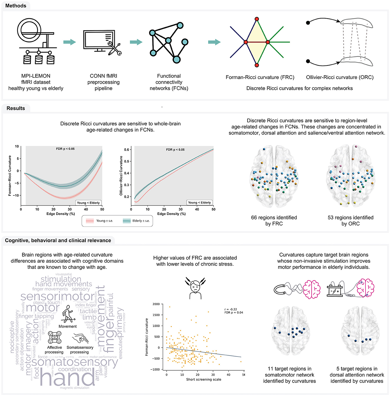
In the present work, we apply FRC and ORC to compare resting-state FCNs of healthy young and healthy elderly individuals. We constructed resting-state FCNs by applying a standard fMRI preprocessing pipeline (Elumalai et al., 2022) to raw rs-fMRI images of 225 healthy participants in the MPI-LEMON dataset (Babayan et al., 2019). We estimated whole-brain and region-level FRC and ORC differences between the young and elderly age groups. Next, we used meta-analysis decoding (Yarkoni et al., 2011; Williams et al., 2021) to determine whether discrete Ricci curvatures can identify the cognitive and behavioral domains that are typically associated with healthy aging. Finally, we performed two post-hoc analyses based on the results of the meta-analysis decoding. For the first post-hoc analysis, we determined whether the node curvatures of brain regions with age-related differences were correlated with performance in behavioral tests of affective processing. Affective processing is known to change with age (Mather, 2012). For the second post-hoc analysis, we compared the set of brain regions showing age-related curvature differences, to the set of brain regions whose non-invasive stimulation with tDCS, tACS, or TMS is known to improve motor performance in healthy older adults. Motor performance is also known to change with age (Seidler et al., 2010; Cirillo, 2021). Figure 1 provides a summary of the methods and the main results obtained in this work.

Figure 1. Summary of workflow and main results obtained in this study. Raw rs-fMRI scans of young participants and elderly participants were obtained from the MPI-LEMON dataset and preprocessed using the CONN toolbox. The preprocessed rs-fMRI scan of each participant was used to construct resting state functional connectivity networks (FCNs) at varying edge densities. Next, we computed and compared Forman-Ricci curvature (FRC) and Ollivier-Ricci curvature (ORC) across the FCNs of the young and elderly groups. We found that both FRC and ORC show whole-brain and region-level differences in the FCNs of young and elderly participants. Additionally, we found that age-related differences in FRC and ORC are associated with the cognitive domains of movement, affective processing and somatosensory processing. Notably, node FRC shows a significant negative correlation with behavioral test scores of chronic stress. Finally, we showed that FRC and ORC can capture brain regions whose non-invasive stimulation is known to improve motor performance of older adults.

2. Materials and methods

We applied Forman-Ricci curvature (FRC) and Ollivier-Ricci curvature (ORC) to measure age-related changes in resting-state functional connectivity networks (FCNs). We constructed the FCNs from raw rs-fMRI images of the subjects acquired from the MPI-LEMON dataset (Babayan et al., 2019). We used the CONN functional connectivity toolbox (Whitfield-Gabrieli and Nieto-Castanon, 2012) to spatially and temporally preprocess the raw rs-fMRI images. Next, we parcellated each preprocessed image into 200 regions of interest (ROIs) or nodes using the Schaefer atlas (Schaefer et al., 2018) and generated a 200 × 200 functional connectivity (FC) matrix for each subject. We constructed the FCNs for each subject using a two-step filtering approach, comprising maximum spanning tree (MST) followed by sparsity-based thresholding. Note that the preprocessing pipeline for raw rs-fMRI images and methodology used to construct the FCNs in this work is identical to our previous work on autism spectrum disorder (Elumalai et al., 2022). In the following, we describe in detail, the procedure we employed to construct and analyze the FCNs.

2.1. Participants and imaging dataset

We obtained raw rs-fMRI and anatomical data for 228 participants from the MPI-LEMON dataset (Babayan et al., 2019), comprising 154 young individuals from 20 to 35 years, and 74 elderly individuals from 59 to 77 years. Middle-aged individuals are not included in the MPI-LEMON dataset. We downloaded all the raw rs-fMRI and anatomical data from the “Functional Connectomes Project International Neuroimaging Data-Sharing Initiative/Child Mind Institute” available at the following link: http://fcon_1000.projects.nitrc.org/indi/retro/MPI_LEMON.html. Further, demographic information of the participants such as handedness, formal education, drug test results, smoking status, relationship status, blood sample, blood pressure, and anthropometry is readily available at the following link: https://ftp.gwdg.de/pub/misc/MPI-Leipzig_Mind-Brain-Body-LEMON/.

Next, we excluded the subjects with corrupted or missing raw files in the MPI-LEMON dataset, resulting in 225 subjects (young group: 153 subjects, elderly group: 72 subjects) that we included for subsequent analyses. Note that the participants included in the MPI-LEMON dataset provided written informed consent prior to any data acquisition, including agreement to share their data anonymously.

2.2. Raw fMRI data preprocessing

We preprocessed the raw rs-fMRI scans from the MPI-LEMON dataset using the CONN functional connectivity toolbox (Whitfield-Gabrieli and Nieto-Castanon, 2012). The preprocessing pipeline used in this study is identical to our previous work on autism spectrum disorder (Elumalai et al., 2022), and we have published earlier a protocol video explaining this pipeline which is available at: https://youtu.be/ch7-dOA-Vlo.

We spatially preprocessed the raw rs-fMRI scans in four major steps: (i) motion correction, (ii) slice-timing correction, (iii) outlier detection, and (iv) structural and functional segmentation and normalization.

For the motion correction step, we co-registered the raw fMRI scans to the first scan of the first session. We corrected the fMRI scans for motion using six rigid body transformation parameters (three translations and three rotations) that are a part of the SPM12 realign and unwarp procedure (Andersson et al., 2001). For the slice-timing correction step, we corrected temporal misalignment between different slices of the fMRI scans using the SPM12 slice-timing correction procedure (Sladky et al., 2011). For the outlier detection step, we used Artifact Detection Tools (ART)-based outlier detection to mark acquisitions as outliers if they were found to have framewise displacement >0.5 mm or global BOLD signal changes >3 standard deviations. For the segmentation and normalization step, we normalized the images into the Montreal Neurological Institute (MNI) space using the standard procedure (Ashburner and Friston, 2005). Subsequently, we segmented the brain into gray matter, white matter and cerebrospinal fluid (CSF) areas using raw T1-weighted volumes of the anatomical scans and mean BOLD signal of the fMRI scans as reference.

With the CONN toolbox, we extracted the BOLD signals (time series) for each voxel after spatially preprocessing the raw rs-fMRI scans, and performed a temporal preprocessing or denoising step to reduce existing motion effects from BOLD signals. First, we applied an anatomical component-based noise correction procedure (aCompCor), which includes a linear regression step. This step resulted in the removal of five possible noise components (Chai et al., 2012) each from white matter and CSF areas, 12 possible noise components due to estimated subject motion parameters and their first-order derivatives (Friston et al., 1996), and 1 noise component from outlier scans detected earlier (scrubbing) (Power et al., 2014). Second, we removed temporal frequencies <0.008 Hz from the BOLD signals using a high-pass filtering approach.

All the 225 subjects passed the quality assessment checks provided by the CONN toolbox (Ciric et al., 2017; see Supplementary Table 1). Finally, we used the preprocessed fMRI scans of these 225 subjects to construct FC matrices and perform network analysis.

2.3. ROI definition and ROI time series estimation

After spatially and temporally preprocessing the raw rs-fMRI scans of the 225 subjects, we partitioned the voxels into cortical parcels so as to define nodes or ROIs with interpretable neurobiological meaning (Luppi and Stamatakis, 2021) and reduce the computational load of further analysis. For this purpose, we used a cortical parcellation atlas provided by Schaefer et al. (2018), which parcellates the brain into 200 distinct ROIs or nodes. Apart from assigning each voxel to one of 200 ROIs, the Schaefer atlas also provides a mapping between each ROI and one of seven resting state networks (RSNs), namely, “default network,” “somatomotor network,” “dorsal attention network,” “salience/ventral attention network,” “visual network,” “limbic network,” and “control network.” With the CONN toolbox, we determined the time series corresponding to each ROI by computing the average time series of its constituent voxels.

2.4. Functional connectivity network construction

We constructed a 200 × 200 FC matrix for each of the 225 subjects, by computing the Pearson correlation coefficient between all pairs of ROI time series. The resulting FC matrix can be considered a complete, weighted, and undirected network with 200 nodes, with the weight of each edge determined by the Pearson correlation coefficient between the time series of its corresponding pair of nodes. We used the FC matrix of each of the 225 subjects to construct the FCNs, using a two-step procedure.

First, we determined the maximum spanning tree (MST) of the FC matrix using Kruskal's algorithm (Kruskal, 1956). The MST for a weighted graph with n nodes is an acyclic graph with (n−1) edges which includes all the nodes of the graph. Using an MST-based filtering approach ensures that the resulting FCN is a connected graph and it captures the highly correlated nodes from the FC matrix.

Second, we used a sparsity-based thresholding procedure, wherein edges from the FC matrix were iteratively added to the MST in decreasing order of their correlation values until we generated a network with the desired edge density. We binarized the thresholded network by removing the edge weights in order to obtain an unweighted, undirected and connected FCN with desired edge density (Achard and Bullmore, 2007; Rudie et al., 2013). Using a sparsity-based filtering approach ensures that the resulting FCNs for different subjects have the same number of edges, which enables a direct mathematical comparison of discrete Ricci curvatures and other network properties across subjects (Bassett et al., 2012; Rudie et al., 2013; Xu et al., 2016). We remark that such a two-step procedure with MST followed by sparsity-based thresholding was used previously by Achard et al. (2012) and Elumalai et al. (2022) to construct resting-state FCNs from FC matrices.

In this work, we computed discrete Ricci curvatures and other network properties over the range of edge densities 0.02–0.5 or 2–50% edges, with an increment of 0.01 or 1% edges (Rudie et al., 2013; Itahashi et al., 2014; Harlalka et al., 2018). Therefore, we constructed 49 FCNs for each of the 225 subjects from the MPI-LEMON dataset. We have made all the 200 × 200 FCNs for 225 subjects across 49 edge densities or thresholds publically available via a GitHub repository: https://github.com/asamallab/Curvature-FCN-Aging.

2.5. Discrete Ricci curvatures

Each FCN generated in our work can be represented as an unweighted and undirected graph or network G = (V, E), where V is the set of vertices or nodes in G and E is the set of edges or links in G. Classically, Ricci curvature is defined on tangent vectors on smooth manifolds (Jost, 2017), whereas for discrete objects such as networks, Ricci curvature is naturally defined on the edges. While both FRC (Forman, 2003; Sreejith et al., 2016) and ORC (Ollivier, 2007) are discrete analogs of the classical Ricci curvature, the definitions for FRC and ORC are non-equivalent, and therefore, the two discrete versions capture distinct properties of the classical Ricci curvature. Notably, FRC captures the geodesic dispersal property of the classical Ricci curvature whereas ORC captures the volume growth property of the classical Ricci curvature (Samal et al., 2018). Below, we present definitions of the two notions of discrete Ricci curvature, specific to an unweighted and undirected network, employed in our work.

2.5.1. Forman-Ricci curvature

Forman (2003) introduced a discretization of Ricci curvature for a particular class of geometric objects known as CW complexes, which are widely studied within the field of algebraic topology. Some of us adapted the notion of Forman-Ricci curvature (FRC) to undirected graphs (Sreejith et al., 2016), which are equivalent to 1-dimensional CW complexes. However, a remarkable property of Forman's discretization is that it can be defined for CW complexes in any arbitrary number of dimensions, which allows for a rigorous means to account for higher-order interactions in complex systems. Notably, we utilized this property in a subsequent work (Samal et al., 2018) and defined a modified version of FRC, also known as augmented FRC. Formally, consider a graph G where weights are assigned to vertices, edges and triangular faces (that is, cycles of length 3). We refer to a vertex, an edge or a triangular face in G as a cell. Every cell in G can be assigned with a dimension. Specifically, vertices have dimension 0, edges have dimension 1 and triangles have dimension 2. The augmented FRC of an edge e in G can then be defined as

F(e)=we[(∑e<fwewf+∑v<ewvwe)         −∑e^∥e|∑e^,e<fwe·we^wf−∑v<e^,ewvwe·we^|]

where we is the weight of edge e, wv is the weight of vertex v, wf is the weight of triangular face f.

For any two cells σ and τ in G, σ <τ denotes that σ is contained in τ. In other words, σ is a lower dimensional cell of τ. Specifically, for an edge e and a triangular face f, e<f means that the triangular face f contains the edge e as one of its sides. Moreover, for a vertex v and an edge e, v<e means that the edge e is anchored on the vertex v.

Any two cells with the same dimension can either share a higher dimensional cell or a lower dimensional cell. For example, two vertices v1 and v2 share an edge e if the edge e connects the vertices v1 and v2. On the other hand, two edges e1 and e2 share a vertex v if both e1 and e2 are anchored at v. Finally, two edges e1 and e2 share a triangular face f, if e1 and e2 are the sides of the triangle f.

Two cells of the same dimension are said to be parallel if they either share a higher dimensional cell or a lower dimensional cell, but not both. For example, two edges e1 and e2 are parallel by definition if they belong to the same triangular face or if they are anchored on the same vertex, but not both. ê∥e denotes the set of edges that are parallel to the edge e.

Augmented FRC accounts for cycles of length 3 in a graph while neglecting cycles of length 4 or higher. We refer the reader to Samal et al. (2018) for a systematic investigation of augmented FRC. If the graph G is unweighted, then all the vertices, edges, and triangular faces are assigned weight equal to 1, and the augmented FRC reduces to the following simple combinatorial expression

F(e)=4-deg(i)-deg(j)+3×tri(e)

where deg(i) and deg(j) are the degrees of nodes i and j, respectively, that are anchored to the edge e and tri(e) is the number of triangular faces that contain the edge e. We refer to augmented FRC simply as FRC throughout the main text. Intuitively, FRC quantifies the extent of the spread of information around the ends of an edge in a network. A more negative value of FRC of an edge indicates a higher amount of information spread around its ends.

2.5.2. Ollivier-Ricci curvature

For an edge e between nodes i and j in an unweighted and undirected graph G, ORC is measured by comparing the minimal cost of transporting a mass distribution over the neighbors of i and j with the distance between i and j itself (Ollivier, 2007; Ni et al., 2015). Formally,

where mi and mj are the discrete probability measures defined on nodes i and j, respectively, and d(i, j) is the distance between i and j. Since G is an unweighted graph, d(i, j) is equal to the number of edges contained in the shortest path connecting i and j. W1 is the transportation distance between mi and mj, also known as the Wasserstein distance (Vaserstein, 1969), which is defined as

W1(mi,mj)=infμi,j∈∏(mi,mj)∑(i′,j′)∈V×Vd(i′,j′)μi,j(i′,j′),

where ∏(mi, mj) is the set of probability measures μi, j that satisfy

∑j′∈Vμi,j(i′,j′)=mi(i′),∑i′∈Vμi,j(i′,j′)=mj(j′).

The above equation gives all the possible transportations of measure mi to mj. The Wasserstein distance W1(mi, mj) is the minimal cost of transporting mi to mj. The probability distribution mi is considered to be uniform over the neighboring nodes of i (Lin et al., 2011). Note that the computation of ORC can be formulated as a linear programming problem (Ni et al., 2015).

2.6. Global and node-level network analyses

For each of the 225 subjects in the MPI-LEMON dataset included in this study, we generated 49 unweighted and undirected FCNs with varying edge densities from 2 to 50% with an increment of 1%. Subsequently, we compared the global or whole-brain characteristics of the FCNs, at each edge density, across the two groups (young and elderly) using FRC and ORC. Specifically, we computed the average FRC of edges and average ORC of edges, for each of the 49 networks, for each of the 225 subjects included in this study. Additionally, we computed eight other global network measures namely, clique number, average clustering coefficient, global efficiency (Latora and Marchiori, 2001), average node betweenness centrality, average local efficiency (Latora and Marchiori, 2001), average shortest path length, modularity (Blondel et al., 2008), and assortativity. We provide the definitions of theses global network measures used to characterize the FCNs in the Supplementary material.

Next, we compared the node or region-level characteristics of the FCNs, at each edge density, across the young and elderly groups. Specifically, we computed the node FRC and node ORC for the 200 nodes, for each of the 49 networks, for each of the 225 subjects included in this study. The notion of node Ricci curvature is analogous to the notion of scalar curvature in Riemannian geometry (Jost, 2017) and is computed as the sum of the Ricci curvatures for the edges incident on a given node (Samal et al., 2018).

The computer codes used to compute the global and node-level network characteristics including FRC and ORC are publicly available via a GitHub repository: https://github.com/asamallab/Curvature-FCN-Aging. The standard network measures were computed using the Python package NetworkX (Hagberg et al., 2008).

2.7. Neurosynth meta-analysis decoding

In order to determine the cognitive and behavioral relevance of the results from node-level comparisons across the young and elderly groups, we used Neurosynth meta-analysis decoding (Yarkoni et al., 2011; Williams et al., 2021). First, we used the Neurosynth meta-analysis tool to find terms related to cognition, perception and behavior corresponding to the centroid coordinates of each of the 200 Schaefer ROIs. Second, we assigned each of the nodes or ROIs with significant between-group differences in FRC or ORC to their respective RSN, as defined by the Schaefer atlas. The ROIs were assigned to one of seven such RSNs, since the Schaefer atlas is divided into seven RSNs. Third, for a given RSN, we computed the number of occurrences of the terms associated with the significant ROIs within that RSN. Fourth, we determined the statistical significance of the number of occurrences of the different terms associated with each RSN. Note that the above steps were performed separately for each RSN.

2.8. Statistical analyses

We employed a two-tailed two-sample t-test to estimate the differences in average edge curvatures and other global network measures between the young and elderly groups throughout the 49 FCN densities in the range 2–50% considered in this work. In order to estimate the between-group differences in node curvatures, we first computed the area under the curve (AUC) for the FRC or ORC of a given node across the 49 edge densities (Achard and Bullmore, 2007; Itahashi et al., 2014). Subsequently, we employed a two-tailed two-sample t-test on the AUCs of the discrete curvatures for each of the 200 nodes of the FCNs.

In order to determine the statistical significance of the number of occurrences of each term in the Neurosynth meta-analysis decoding, we first computed the number of occurrences of the same terms corresponding to equal number of randomly selected nodes (surrogate ROIs). For example, if we identified 66 nodes with significant between-group differences in FRC, then we randomly selected a set of 66 nodes out of the 200 nodes in the Schaefer atlas. We obtained a null distribution for the number of occurrences of each term by generating 1,000 sets of randomly selected nodes. Subsequently, we calculated the z-score corresponding to the number of occurrences of each term associated with the subset of original ROIs. Finally, we converted the z-scores to p-values, assuming a normal distribution (Williams et al., 2021; Elumalai et al., 2022).

In order to correct for multiple comparisons and control the occurrence of false positives, we employed a false discovery rate (FDR) correction (Benjamini and Hochberg, 1995) to adjust the p-values for each of the statistical tests described above. We set the threshold α for these FDR corrections to 0.05. These statistical tests were performed using Python packages SciPy (Virtanen et al., 2020) and statsmodels (Seabold and Perktold, 2010). No covariates were used in the statistical analyses.

2.9. Correlation of node curvatures with cognitive and behavioral scores

Neurosynth meta-analysis decoding revealed cognitive and behavioral domains associated with those brain regions whose node curvatures were different between young and elderly participants. We performed a correlation analysis to determine the extent to which curvatures of individual brain regions could account for variation in performance on tests measuring ability in cognitive or behavioral domains linked to those regions. Specifically, if the Neurosynth meta-analysis for a given RSN revealed a particular cognitive or behavioral domain, then we acquired all the phenotypic test scores associated with that domain for each of the 225 subjects in the MPI-LEMON dataset. Note that the MPI-LEMON dataset contains detailed information on 6 cognitive tests and 21 questionnaires related to emotional behavior, personality traits and tendencies, eating behavior, and addictive behavior. This data can be accessed via the links https://ftp.gwdg.de/pub/misc/MPI-Leipzig_Mind-Brain-Body-LEMON/ or http://fcon_1000.projects.nitrc.org/indi/retro/MPI_LEMON.html.

Next, we computed Spearman's correlation between the node FRC (or node ORC) of all the significant regions in that RSN and the phenotypic scores provided in each of the cognitive or behavioral tests. We used Spearman rather than Pearson correlation since some of the test scores are expressed on an ordinal rather than continuous scale. Finally, we performed FDR correction to adjust the p-values of the estimated correlations. FDR correction was applied to p-values of each cognitive or behavioral test, separately. Note that if a particular cognitive or behavioral test had multiple phenotypic scores, then the FDR correction was applied across all the phenotypic scores within that test.

2.10. Literature search of non-invasive brain stimulation studies in healthy elderly individuals

We performed a literature search on PubMed to identify scientific papers reporting the effect of three non-invasive brain stimulation techniques namely, tDCS, tACS, and TMS on motor performance in healthy elderly individuals. Then, we assessed the results reported in these papers to identify brain regions that show evidence for improvements in motor performance of elderly individuals after non-invasive stimulation. The following search query was used in PubMed: [(transcranial magnetic stimulation) OR (TMS) OR (transcranial direct current stimulation) OR (tDCS) OR (transcranial alternating current stimulation) OR (tACS)] AND [(healthy old) OR (healthy elderly) OR (healthy aging) OR (healthy aging)] AND [(motor function) OR (motor performance) OR (motor skill) OR (movement)]. This PubMed search was performed in October 2022, and returned a list of 1,659 articles.

We followed a three-stage procedure to identify relevant articles from the list of 1,659 articles returned by the PubMed search (see Supplementary Figure 1). First, we checked all the meta-analysis papers studying the effects of tDCS, tACS, or TMS on motor performance in elderly individuals (Summers et al., 2016; Patel et al., 2019; Lee et al., 2021; Pino-Esteban et al., 2021) to identify articles that were missing from the list of 1,659 articles. Second, we filtered the relevant articles from the list of 1,659 articles based on title and abstract. Third, we classified the articles according to the non-invasive stimulation technique employed (tDCS, tACS, or TMS) and checked the full text of the articles for relevance. We used the following inclusion criteria to judge article relevance: (1) studies on healthy elderly individuals, (2) studies that employ non-invasive brain stimulation, namely tDCS, tACS, and TMS, (3) studies that analyze the effect of non-invasive stimulation techniques on motor performance, as measured during movement-related tasks such as finger tapping tasks (FTT), sequence learning tasks and serial reaction time tasks (SRTT), and their variants, and (4) studies that are peer-reviewed. We used the following exclusion criteria to judge article relevance: (1) review articles, (2) articles presented in languages other than English, (3) studies that did not employ non-invasive stimulation, (4) studies that investigate new protocols for brain stimulation, (5) studies on diseased populations, including patients with Alzheimer's Disease, Parkinson's Disease or Stroke, (6) studies on non-human species, e.g., rats, (7) studies that employed non-invasive stimulation on children or young adults, (8) studies that analyze the effect of non-invasive stimulation on domains other than motor performance, and (9) studies that analyze the effect of non-invasive stimulation on neuronal activity, neuroplasticity or neurophysiological processes. A given article was considered as relevant only if all the inclusion criteria were satisfied, whereas it was considered as not relevant if at least one exclusion criterion was satisfied.

The above procedure resulted in 36 eligible articles that employed tDCS, three eligible articles that employed tACS, and two eligible articles that employed TMS in their experiments. We extracted the following data from the eligible articles: PMID, author, publication year, participant information (which includes number of participants and mean age of the participants), type of stimulation (for example, anodal tDCS, cathodal tDCS, bilateral tDCS, rTMS), target brain region, stimulation parameters (such as stimulation intensity for tDCS and tACS, pulses per session and inter-train interval for TMS, number of sessions, and treatment duration), outcome measures used to assess motor performance after stimulation, results of stimulation, and adverse effects of stimulation on experimental group or control group (if applicable). Supplementary Table 2 provides the data extracted from the tDCS, tACS, and TMS studies, respectively. From the above data, we combined information about the target region, outcome measures and results of tDCS/tACS/TMS stimulation as measured using the outcome measures in each study to identify the set of target regions whose non-invasive stimulation resulted in improved motor performance of healthy older individuals. These target regions were used in a subsequent analysis to determine whether FRC or ORC can identify brain regions whose non-invasive stimulation shows evidence for improvements in motor performance of healthy older individuals.

2.11. Determining overlap between brain regions with age-related differences in curvature and target regions in non-invasive stimulation studies

Next, we performed a systematic comparison of the age-related differences in discrete Ricci curvatures with results from previous non-invasive stimulation studies. However, note that the target regions in our collected list of non-invasive brain stimulation experiments correspond to the ROIs in the Brodmann atlas (Strotzer, 2009), whereas the brain regions with age-related differences in FRC or ORC correspond to the ROIs in the Schaefer 200 atlas. Therefore, in order to enable such a comparison, we merged the two atlases together and subsequently determined the overlap between brain regions with age-related differences in curvature and target regions of non-invasive brain stimulation experiments. More precisely, we employed the following two-step procedure. First, we mapped each Schaefer ROI to a corresponding Brodmann ROI. The mapping was performed using the MRIcron tool (Rorden et al., 2007) by identifying the Brodmann area that contains the MNI centroid coordinates of a given Schaefer ROI. We remark that a similar mapping approach was employed in our previous study (Elumalai et al., 2022) where some of us applied discrete Ricci curvatures to identify brain regions related to atypical functional connectivity in ASD. Second, we determined the set of Brodmann ROIs corresponding to the target regions in non-invasive brain stimulation experiments that show evidence for improvements in motor performance in healthy elderly. Third, we identified the set of Schaefer ROIs that were mapped to these Brodmann ROIs. Fourth, we identified the Schaefer ROIs within this set that also showed significant age-related differences in FRC or ORC.

3. Results

In this work, we employed two geometry-inspired graph measures namely, FRC and ORC, to investigate the whole-brain and region-level differences in resting state FCNs during healthy aging. We preprocessed raw rs-fMRI images of 153 healthy, young individuals in the age range 20–35 years and 72 healthy, elderly individuals in the age range 59–77 years from the MPI-LEMON dataset. Next, we used the Schaefer atlas (Schaefer et al., 2018) to parcellate the preprocessed rs-fMRI scan of each subject into 200 ROIs, and calculated the Pearson correlation coefficient between all pairs of ROI time series, yielding a 200 × 200 FC matrix. Finally, we generated 49 FCNs for each subject across the range of edge densities 0.02–0.5 or 2–50% edges, with an increment of 0.01 or 1% edges using a two-step edge filtering approach comprising MST and sparsity-based thresholding. The detailed methodology to construct and analyze the FCNs is described in Section 2.

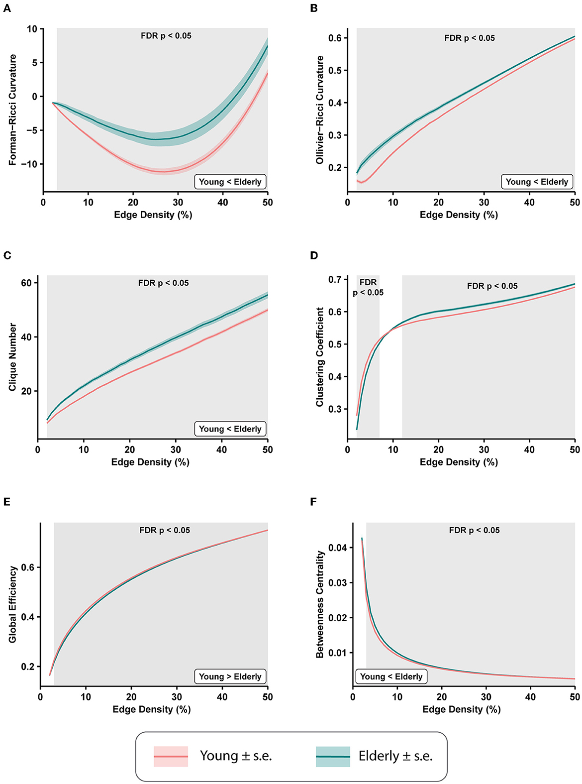
3.1. Whole-brain differences in functional connectivity networks

We computed the average edge FRC and average edge ORC for the 49 FCNs across edge densities 2–50% for each of the 225 subjects to evaluate the age-related brain-wide changes in FCNs between the healthy young and healthy elderly groups. Subsequently, we applied a two-tailed two-sample t-test with FDR correction (see Section 2) to estimate the differences in average edge curvatures between the young and elderly groups at each value of edge density. Figures 2A, B show the differences in average edge FRC and average edge ORC, respectively, between the young and elderly individuals over the range of edge densities 2–50%. We found that the elderly group had significantly higher values of average edge FRC (p < 0.05, FDR-corrected) over the range of edge densities 3–50% (Figure 2A). Similarly, we found that the elderly group had significantly higher values of average edge ORC over the entire range of edge densities 2–50% considered in this study (Figure 2B).

Figure 2. Differences in average edge curvatures and standard global network measures across the functional connectivity networks (FCNs) of 153 young individuals and 72 elderly individuals from the MPI-LEMON dataset. The differences are reported for FCNs over the range of edge densities 0.02 (i.e., 2% edges) and 0.5 (i.e., 50% edges), with an increment of 0.01 (i.e., 1% edges). The shaded regions in each plot correspond to the edge densities where the between-group differences are statistically significant (p < 0.05, FDR-corrected). (A) Average Forman-Ricci curvature (FRC) of edges is higher in elderly individuals over edge densities 3–50%. (B) Average Ollivier-Ricci curvature (ORC) of edges is higher in elderly individuals over the entire range of edge densities considered (2–50%). (C) Clique number is higher in elderly individuals over all edge densities 2–50%. (D) Average clustering coefficient is higher in young individuals over edge densities 2–7%, and higher in elderly individuals over edge densities 12–50%. (E) Global efficiency is reduced in elderly individuals over edge densities 3–50%. (F) Average node betweenness centrality is higher in elderly individuals over edge densities 3–49%.

We further compared eight other global network measures to evaluate brain-wide changes in FCNs of young and elderly individuals. The eight global network measures include clique number, average clustering coefficient, global efficiency, average node betweenness centrality, average local efficiency, shortest path length, modularity, and assortativity. Out of the eight measures, clique number, node betweenness centrality, and assortativity have not been applied in previous network-based analyses of rs-fMRI scans in healthy aging. First, we found that the clique number is significantly higher in elderly group (p < 0.05, FDR-corrected) over all edge densities considered in this study (Figure 2C). Second, we found average clustering coefficient is significantly higher in the young group at edge densities 2–7%, whereas it is significantly higher in the elderly group at edge densities 12–50% (Figure 2D). This change in the directionality of the differences in clustering coefficient with increasing edge densities suggests that highly correlated nodes or ROIs tend to cluster in young individuals whereas weakly correlated nodes tend to cluster in elderly individuals. Notably, the group differences in clustering coefficient observed in the present work are consistent with previous studies that have used clustering coefficient to compare the global changes in resting state FCNs in healthy aging cohorts (Sala-Llonch et al., 2014; Li et al., 2016). Third, we found that global efficiency of the FCNs is significantly reduced in elderly individuals over the edge density range 3–50% (Figure 2E), and our results are consistent with previous graph-theoretic rs-fMRI studies (Achard and Bullmore, 2007; Sala-Llonch et al., 2014; Song et al., 2014; Geerligs et al., 2015; Li et al., 2016) in healthy aging populations. Fourth, we found that average node betweenness centrality of the FCNs is significantly higher in elderly individuals over the edge density range 3–49% (Figure 2F).

Fifth, we found that average local efficiency is significantly higher in the FCNs of the young group compared to the elderly group over the edge density range 1–12%, and significantly higher in the elderly group over the edge density range 19–49% (Supplementary Figure 2). Notably, the differences in average local efficiency observed in the present work are consistent with previous graph-theoretic rs-fMRI studies (Achard and Bullmore, 2007; Song et al., 2014; Geerligs et al., 2015) in healthy aging populations. Sixth, we found that average shortest path length is significantly higher in the elderly group over the edge density range 3–50% (Supplementary Figure 2), and these differences are consistent with previous graph-theoretic rs-fMRI studies (Sala-Llonch et al., 2014) in healthy aging populations. Seventh, we found that modularity is significantly reduced in elderly individuals over the range of edge densities 2–9% (Supplementary Figure 2), and these differences are consistent with results from previous graph-theoretic rs-fMRI studies (Song et al., 2014; Geerligs et al., 2015) in healthy aging populations. Eighth, we found that assortativity is reduced in the elderly group, but the differences are not significant (as suggested by p>0.05, FDR-corrected).

Supplementary Table 3 lists the FDR-corrected p-values corresponding to the group-wise comparisons of discrete Ricci curvatures and standard network measures across all edge densities 2–50% considered in this study.

3.2. Region-level differences in functional connectivity networks

As reported in the previous subsection, we found that both FRC and ORC show significant differences between the resting state FCNs of young and elderly individuals at the whole-brain level. Subsequently, we determined how the global differences in discrete Ricci curvatures are distributed across the 200 nodes or ROIs in the brain as defined by the Schaefer atlas (see Section 2). First, for each of the 225 subjects, we computed node FRC and node ORC for the 200 nodes in the 49 FCNs across the range of edge densities 2–50%. Second, in order to determine the nodes with significant between-group differences in node Ricci curvatures in the FCNs of young and elderly individuals, we computed the Area Under Curve (AUC) of the node curvature values across the 49 edge densities for each of the 200 nodes, and compared these AUCs for each node using a two-tailed two-sample t-test with FDR correction.

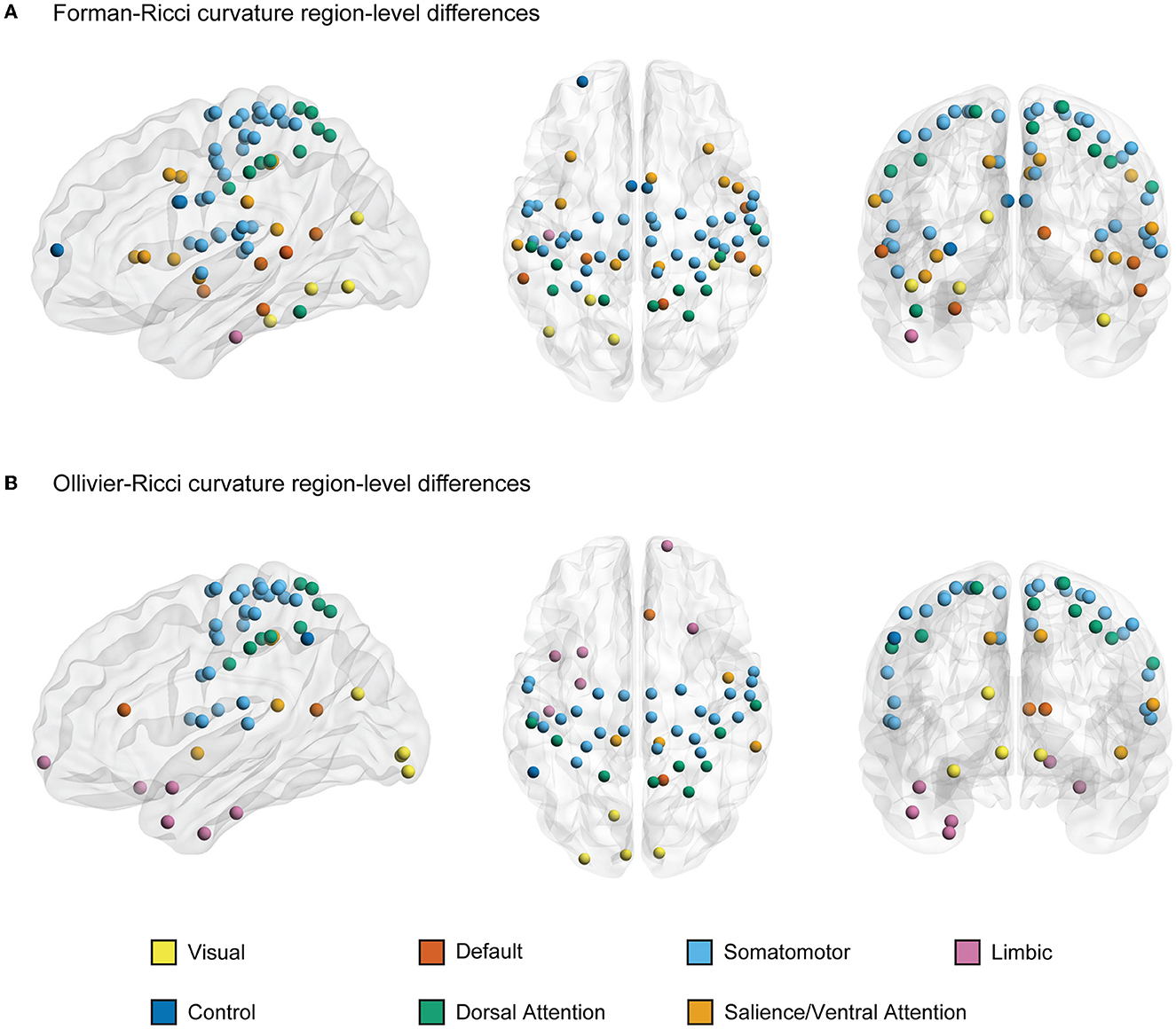
Figures 3A, B illustrate the nodes or ROIs that display significant between-group differences (p < 0.05, FDR-corrected) in FRC and ORC, respectively, of the FCNs of young and elderly individuals. We identified 66 ROIs with significant differences in FRC and 53 ROIs with significant differences in ORC across the young and elderly groups. We found 42 ROIs to be identified by both FRC and ORC. We found that the significant ROIs identified by both FRC and ORC are spread across the 7 RSNs. However, the ROIs with significant differences in node FRC are concentrated in 3 RSNs namely, somatomotor network (33 ROIs), salience/ventral attention network (10 ROIs) and dorsal attention network (10 ROIs). The ROIs with significant differences in node ORC are concentrated in 2 RSNs namely, somatomotor network (27 ROIs) and dorsal attention network (9 ROIs). Supplementary Table 4 lists the ROIs with significant between-group differences as identified by FRC and ORC, partitioned across the 7 RSNs.

Figure 3. A visual representation of nodes or regions in the brain that show significant differences in discrete Ricci curvatures between the functional connectivity networks (FCNs) of young and elderly individuals (p < 0.05, FDR corrected). (A) 66 regions that show significant differences in Forman-Ricci curvature (FRC) of the nodes in the FCNs of the young and elderly groups. All the 66 regions display higher values of node FRC for elderly individuals compared to young individuals. (B) 53 regions that show significant differences in Ollivier-Ricci curvature (ORC) of the nodes in the FCNs of the young and elderly groups. 41 out of these 53 regions display higher values of node ORC in elderly individuals and the remaining 12 ROIs display higher values of node ORC in young individuals. The nodes are specified by the Schaefer atlas, and color-coded as per the 7 resting state networks (RSNs) listed in the figure legend. This figure was created using BrainNet Viewer (Xia et al., 2013). Supplementary Table 5 lists the FDR corrected p-values corresponding to curvature-related differences in each region.