1. Introduction

Schizophrenia (SZ) is a complex challenging mental disorder resulting in significant functional, behavioral, and cognitive impairments (Friston and Frith, 1995; Palmer et al., 1997; Green et al., 2000; Luck and Gold, 2008; Sponheim et al., 2010; Rubinov and Bullmore, 2013). This disorder, which affects about 0.45% of the adult population worldwide (GBD 2016 Disease Injury Incidence Prevalence Collaborators, 2017), is rooted in a combination of genetic and environmental factors; although the exact causes are still unclear. SZ is known as a brain disconnectivity syndrome (Friston and Frith, 1995; Yu et al., 2012; A Ure et al., 2018; McNabb et al., 2018; Li S. et al., 2019), pointing to abnormal interaction between critical areas of the brain. Focusing on connectivity abnormalities, functional magnetic resonance imaging (fMRI) has been increasingly used to study brain dysfunctions in individuals living with SZ (Yu et al., 2012; Dong et al., 2018; Adhikari et al., 2019). Several studies have found evidence for altered resting-state functional connectivity (FC) in different brain regions of SZ people compared to healthy control (HC) subjects (Yu et al., 2012; Karbasforoushan and Woodward, 2013; Dong et al., 2018; Zhuo et al., 2018; Bulbul et al., 2022; Cai et al., 2022). Basically, our various brain functions are generated by its interactive connections. Therefore, exploring brain variations in disorders at the network level can be more helpful in understanding brain functionality alterations in SZ people.

Exploring brain abnormalities in SZ individuals compared to HC can be investigated by a variety of methods at the voxel or regional level. In these studies, regions of interest (ROI) are usually identified through seed-based analysis (Zhou et al., 2007; Whitfield-Gabrieli et al., 2009; Salvador et al., 2010; Woodward et al., 2011; Zhuo et al., 2018; Li S. et al., 2019; Li X.-B. et al., 2019; Gong et al., 2020; Ahmad et al., 2023) or independent component analysis (ICA) (Calhoun and Adali, 2012; Anderson and Cohen, 2013; Lottman et al., 2019; Salman et al., 2019; Forlim et al., 2020), and then, the functional activity of desired regions or connectivity strength of each voxel/region pair is compared across SZ and HC (Camchong et al., 2011; Wolf et al., 2011; Mingoia et al., 2012; Yu et al., 2012; Karbasforoushan and Woodward, 2013; Li S. et al., 2019). Moreover, several connectivity parameters of graph theory have been evaluated for the whole brain network, indicating a significant increase in path length in SZ people and a significant decrease in nodal degree, functional connectivity strength, global efficiency, small-worldness, etc. (Liu et al., 2008; Lynall et al., 2010; Micheloyannis, 2012; Anderson and Cohen, 2013; Hadley et al., 2016; Xiang et al., 2020). Overall, the abnormal areas are mostly sought through primary hypotheses or by an overall (random) search of the whole brain. The latter depends on the search algorithm, and the former is limited by the accuracy of prior knowledge.

Regardless of the search algorithm, the findings of previous methods usually report the alterations in some brain regions or some scattered connections, rather than describing them in the form of modulating networks. Such modulating networks have been recently introduced in a study (Keyvanfard et al., 2020), where a blind ICA approach discovered the building blocks (units) of inter-individual brain variations at the network level. It has been shown that each derived building block may participate in the modulation of several brain functions related to inter-subject variations. Introducing more subjects with new variations (caused by the disorder) is expected to result in the formation of new components encompassing the brain variations related to the SZ.

Therefore, the main purpose of this study was to investigate the usability of the previously proposed approach (Keyvanfard et al., 2020) in determining units of inter-group variations between SZ and HC. In the current study, we modify the previously developed algorithm and investigate the alteration of brain connections (subnetworks) due to including the SZ group in addition to the HC group. This modification consists of two steps: improving the component reproducibility and providing a new method of edge pruning (and therefore the number of pruned edges will not be similar for all subnetworks). We also examined how similar the obtained subnetworks are to the well-known resting-state networks (RSNs) (Smith et al., 2009). Through this systematic method of the developed approach, we expect to obtain brain subnetworks that are more sensitive to connection alterations due to SZ. This higher sensitivity could potentially help to introduce new biomarkers or efficient classifiers.

2. Materials and methods 2.1. Participants, data acquisition, and preparation

In this study, we retrospectively used the resting-state functional MRI (rs-fMRI) data of an SZ group of 27 subjects (mean age, 41.9±9.6) and the completely matched control group of 27 healthy individuals [mean age, 35±6.8; datasets are publicly available on the Zenodo platform (Vohryzek et al., 2020)]. The individuals in the SZ group had been recruited from the Service of General Psychiatry at the Lausanne University Hospital. They had met DSM-IV criteria for SZ and schizoaffective disorders (American Psychiatric Association, 2000). Healthy controls had been recruited through advertisement and assessed with the Diagnostic Interview for Genetic Studies (Preisig et al., 1999). Subjects with major mood, psychotic, or substance-use disorders and having a first-degree relative with a psychotic disorder had been excluded. Moreover, a history of neurological diseases was an exclusion criterion for all subjects. The informed written consent had been obtained for all subjects according to the Ethics Committee of Clinical Research of the Faculty of Biology and Medicine, University of Lausanne, Switzerland (#82/14, #382/11, #26.4.2005). For each participant, two types of MR imaging including rs-fMRI and T1-weighted had been acquired using a 3T Siemens Trio Scanner equipped with a 32-channel head coil.

The magnetization-prepared rapid acquisition gradient echo (MPRAGE) sequence had been applied for T1-weighted imaging with a resolution of 1 × 1 × 1.2 mm3 and TI/TE/TR = 900/2.98/2,300 ms. Each rs-fMRI scan had a duration of 8 min with a 3.3 mm isotropic voxel size and TE/TR = 30/1,920 ms. The performed data preprocessing included the exclusion of the first four time points of signal, regressing out of physiological signal (white-matter and cerebrospinal fluid), motion correction, physiological noise correction, spatial smoothing, bandpass filtering, and linear registration to the T1-weighted image.

Employing the Desikan Killiany atlas (Desikan et al., 2006) and extra parcellation of the cortical surface described in Cammoun et al. (2012), the gray matter of each subject in MPRAGE volume had been partitioned into 129 cortical regions of interest (ROI) including 114 cortical ROIs and 14 subcortical nuclei plus the brain stem. These brain regions had been used to estimate the functional connectivity matrices based on the Pearson correlation between individual brain regions' time courses. Finally, one functional connectivity matrix with the dimension K×K (with K = 129 number of the brain parcels) had been constructed for each participant [please refer to Vohryzek et al. (2020) for detailed information.] Here, to consider the connections' strength, the absolute value of the Pearson correlation in the functional connectivity matrix was utilized. The functional connectivity matrices were then evaluated for normality through the Shapiro–Wilk test (Shapiro et al., 1968). Their p-value > 0.48 (>>0.05) indicated that they follow a normal distribution.

2.2. PCA and ICA

The lower triangular elements of the FC matrix of each subject were considered for constructing the feature matrix. The elements were reshaped into a one-dimensional vector of the size K(K-1)2, where K = 129 is the number of parcels. Afterward, FC vectors of all subjects were stacked to form the X matrix. Thus, X had N rows; the number of subjects and K(K-1)2 columns. Principal component analysis (PCA) was then performed on the feature matrices along the subject dimension and 90% of data variance was preserved. X′ is the new representation of the original feature matrix after applying PCA. The next step is source extraction from the X′ matrix using the ICA approach as in Eq (1).

where A is the mixing matrix and S is the independent source. ICA was performed based on the Infomax (Bell and Sejnowski, 1995) algorithm. Each row in S is considered one component, whose values determine the contribution of edges in that component. We call these values the “ICA value” of the edges in the rest of this study. A few of these components have a major role in forming the feature matrix X′. Selecting the important components among all of them requires an algorithm to assess the reproducibility of the components during different runs. Ranking and Averaging Independent Component Analysis by Reproducibility (RAICAR) (Yang et al., 2008) had been previously employed (Keyvanfard et al., 2020) to avoid run-to-run variability of components ordering and identify reproducible components across 100 ICA runs. Nevertheless, the edge value of obtained (ordered) components in RAICAR was averaged and therefore varied during different runs, and it resulted in dissimilar final subnetworks in different runs. To overcome this limitation, we modified the RAICAR algorithm by considering the correlation values as well as the number of similar components, so that every time, it resulted in the same components with no need to average or perform any kind of manipulation of the edge values. Details are discussed in section 1 of the Supplementary material.

2.3. Edge pruning

The components derived from ICA consist of all brain connections with different weights (the ICA values). Edge pruning is, therefore, required in order to keep only the important connections. This had been previously performed through their z-score values (normalization of connections of each component by subtracting the mean value of that component and dividing by its standard deviation) and thresholding them (Keyvanfard et al., 2020). This would result, however, in having a similar number of connections remaining in each component (due to their normal distribution). Here, we modified the pruning algorithm by revisiting the definition of importance for each edge. In the previous criterion (based on z-score), the weight values of edges specified their importance level. Here, their effect on the reversibility of the ICA procedure was replaced instead of that criterion. We, therefore, developed a new algorithm (detailed in section 2 of the Supplementary material) to calculate the contribution of each edge to the reconstruction of the original functional connectivity matrices. The edges with maximum effects on the reversibility of the ICA procedure were kept, and the others were replaced by zero. The component after edge pruning will be hereafter referred to as a “subnetwork.”

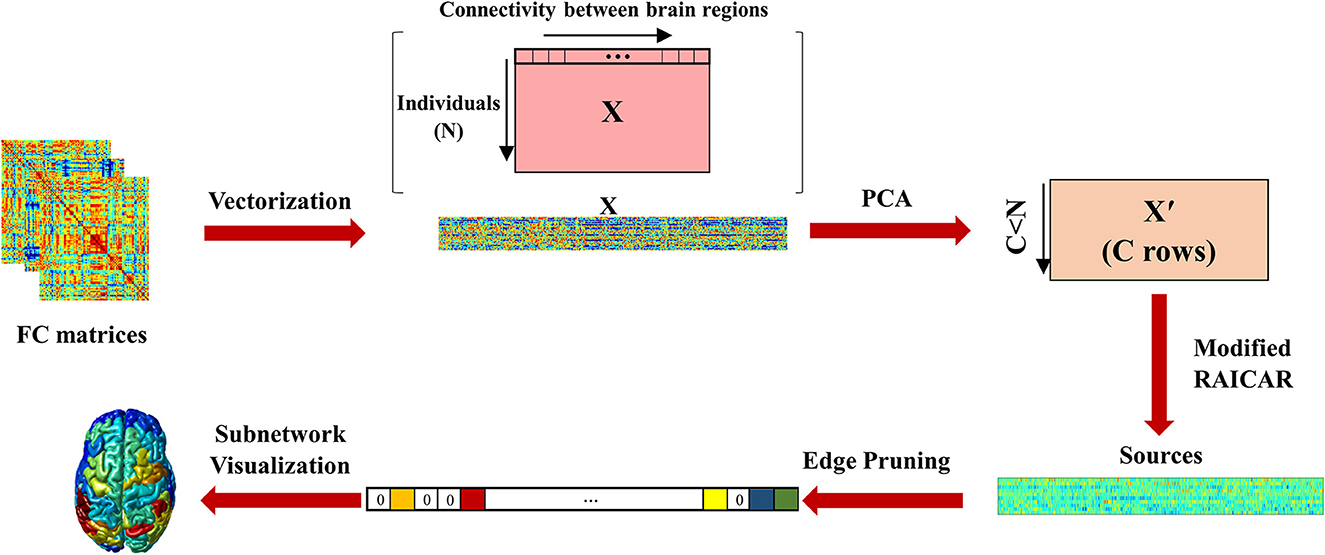
The pipeline of the proposed algorithm is shown in Figure 1.

Figure 1. The proposed pipeline. The functional connectivity matrices of all participants were vectorized and stacked on top of each other. The size of this matrix was N×(K(K-1)2). PCA was performed to reduce information redundancy. The reduced feature matrix had C < N rows. The modified RAICAR algorithm based on Infomax was then applied. Next, edge pruning was performed to select the most important edges in each component (zero edges show pruned connections and the colors indicate different ICA values of edges). Finally, cortical surface maps of functional subnetworks were constructed based on their normalized nodal strengths.

2.4. Statistical analysis

The subnetworks should be statistically evaluated to determine significantly different subnetworks between the HC and SZ groups. To this end, each individual was projected on a vector, which was defined by two different methods as described below. The statistical analysis was then performed on the projected values.

A) In this viewpoint, only the location of preserved connections (rather than the ICA values) was considered on each subnetwork. For the subnetwork i: first, the location of the selected edges was determined. Second, the mean weight of the original functional connectivity values of the selected edges in the HC and SZ groups was calculated. Third, the difference between these two mean vectors was calculated (Diff(i)). Then, for each subject in the two groups, the original functional connectivity vector of selected connections was projected on the difference vector (through the inner product) as follows:

for subnetwork(i):

Diff(i)=|VHC(i)−VSZ(i)|,

for subject(j):

A−PrjHC(i,j)= 〈Diff(i) , FCHC(i,j)〉   A−PrjSZ(i,j)=〈Diff(i) , FCSZ(i,j)〉    (2)

where V is the average vector of FC values of subnetwork i, FC (i,j) is the functional connectivity vector of individual j at the location of selected connections in subnetwork i, and 〈x, y〉 illustrates the inner product of x and y vectors. Finally, a two-sample t-test was applied between the obtained projected vectors, A−PrjHC(i) and A−PrjSZ(i ).

B) Since some selected locations were common among different subnetworks, in this comparison, we were interested in giving value to the degree of contribution of each edge. In other words, the ICA values of the selected edges in the subnetworks were considered. The functional connectivity weights of each individual were projected on the subnetworks through the inner product. Statistical analysis was then applied between these projected values of the two groups (B−PrjHC,B−PrjSZ). Here, functional connectivity averaging is no longer performed over individuals and is, therefore, expected to be more robust against inter-individual variations within a group.

for component(i)and subject(j):

B−PrjHC(i,j)= 〈Comp(i) , FCHC(j)〉    B−PrjSZ(i,j)=〈Comp(i) , FCSZ(j)〉    (3)

The Bonferroni correction (Benjamini and Hochberg, 1995) for multiple comparisons was employed for both parts, A and B, and the p-value < 0.005 was considered statistically significant.

Furthermore, the practical significance of the outcomes was evaluated through the calculation of the effect size. Cohen's d, the most common measurement method of effect size was used, where the mean difference between the two groups is divided by the pooled standard deviation.

2.5. Components evaluation

The distribution of connectivity values for the subnetworks that significantly differentiated the SZ group from HC, and called “significant subnetworks” hereafter, was compared with the well-known RSNs introduced by Yeo et al. (2011). Yeo's atlas includes seven RSNs: visual (VIS), somatomotor (SM), dorsal attention (DA), ventral attention (VA), frontoparietal (FPN), default mode network (DMN), and limbic (Limb) functional systems. These RSNs are illustrated in Supplementary Figure 2. The overlap between the subnetworks and the seven RSNs was determined by computing nodal strengths summation of the common nodes between the RSNs and the obtained subnetworks (Keyvanfard et al., 2020). The detail can be found in section 4 of the Supplementary material.

A non-parametric permutation test was used to statistically evaluate the overlap percentage between the subnetworks and the RSNs. To this end, connection weights were randomly assigned to each subnetwork and the overlap percentage with the RSNs was recalculated. This procedure was repeated 1,000 times. The p-value was then computed as the number of times that the newly obtained overlap percentage exceeded the test statistic obtained from the original data, divided by the number of permutations. The significance level was set to 0.005.

2.6. Graph parameters

We performed graph theory analysis to examine the connectivity characteristics of the whole brain network as well as the obtained subnetworks. The whole brain network analysis was conducted on weighted and fully connected FC matrices of each individual. In other words, no thresholding and binarization were applied to the adjacency matrices. The five common topological measures were computed: shortest path length, network strength, global and local efficiency, and clustering coefficient, and then, t-test statistical analysis was applied between these graph measures of the two groups, HC and SZ.

In the next step, the graph theory analysis was performed on the obtained subnetworks. For each individual, the weighted subnetwork graph was constructed based on the original functional connectivity values at the location of the selected edges. The same five graph metrics were calculated and then statistically analyzed to determine significant differences between SZ and HC groups.

All graph theoretic measures for the weighted graphs were computed with the Brain Connectivity Toolbox (Rubinov and Sporns, 2010). In this section, a p-value < 0.05 was considered to indicate statistical significance.

The graph topological characteristics utilized in this study are described as follows:

The shortest path length of a node pair is the minimum edge weight summation required to link the ith and the jth node. The average of the shortest path length of the network Lnet, or characteristic path length, is the mean of the shortest path length between all node pairs (N) in the network (Watts and Strogatz, 1998):

Lnet = 1N​(N−1)∑i≠ jLij    (4)

Network strength (S) is computed as the average of the nodal strength (defined as the summation of all absolute edge values (wij) connected to each node) of all nodes in the network (Liu et al., 2017). It is described as follows:

S = 1N∑i≠jwij    (5)

Global efficiency (Eglobal) measures the degree of integration of brain networks (Latora and Marchiori, 2001, 2003; Achard and Bullmore, 2007). It is the inverse of the average of the shortest path length between each node pair and is defined as follows:

Eglobal = 1N(N−1)∑​i≠j1min{Li,j}    (6)

The local efficiency (Ei_local) could be interpreted as how well the nodes in the subgraph Gi exchange information when the ith node is removed, revealing the tolerance of the network (Latora and Marchiori, 2001). Its calculation is as follows:

Eilocal = 1NGi(NGi-1)∑i≠j1min    (7)

The absolute clustering coefficient of a node (Ci) in a weighted graph is the ratio of the sum of triangle intensities (wij) to the number of all possible connections in the subgraph Gi including k nodes (Onnela et al., 2005):

Ci = Eiki(ki-1)2 = 2ki(ki-1) ∑j,k(wij, wik,wjk)13    (8)

The clustering coefficient of a network Cnet is then derived by averaging the clustering coefficients of all nodes within the network.

Cnet = 1N∑i∈GCi    (9)

The entire analysis of this study was performed using MATLAB version 2021a.

3. Results

Applying the developed algorithm on the concatenated connectivity matrix of both HC and SZ groups led to obtaining brain subnetworks. Considering the robustness of the components (Keyvanfard et al., 2020) and the connectedness of the areas, only the first eight subnetworks were studied in this study (see Discussion for more details). The edge pruning step was performed with a threshold of 0.2, which resulted in more than 30% of the edges remaining in the subnetworks.

The order of the input data was randomly changed 10 times, and the developed algorithm was re-executed. To assess the change in the order of the output components that might occur due to a change in the order of the input data, we used the correlation coefficient as a similarity index to find the corresponding components in every two runs. The modified RAICAR algorithm resulted in the appearance of all components in their stable locations within 10 times implementation. Moreover, evaluation of the ICA value in each component showed that there was no change in the different runs of the algorithm.

3.1. Statistical analysis

Based on the two types of scoring for statistical analysis, described in section 2.4, a statistical analysis was performed on each subnetwork and the following outcomes resulted:

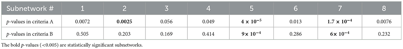
A) Considering the location of selected edges in the subnetworks (see Eq. 2), three of eight, #2 (p = 0.0025), #5 (p = 4 × 10−5), and #7 (p = 1.7 × 10−4) showed a statistically significant difference between HC and SZ people.

B) Subnetwork #5 (p = 9 × 10−4) and #7 (p = 6 × 10−4) significantly differentiated SZ from HC using the ICA values in the projected values (described in criteria B, Eq. 3).

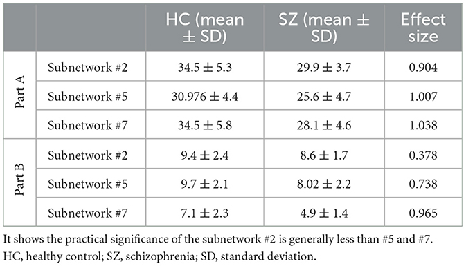
The p-value of all subnetworks is listed in Table 1. The lower p-values of subnetwork #5 and subnetwork #7 in Part A (Table 1) may indicate that they are more specific to the SZ and called the “SZ-specific” subnetworks hereafter. This outcome can be also inferred from p-values in Part B (Table 1) in which considering the ICA values resulted in an increased p-value (to be not significant anymore) for #2. Moreover, the reported effect sizes in Table 2 support this outcome. Cohen's d for #2 in Part A was higher than 0.8 which implied a large impact; however, this value was less than the other two subnetworks. In Part B, the effect size of subnetwork #2 decreased to 0.3, which revealed its almost limited practical application compared to Cohen's d > 0.7 in #5 and #7.

Table 1. p-values of all subnetworks through two types (A and B) of statistical analysis.

Table 2. Effect size of three subnetworks through both statistical analysis, Part A and Part B in section 2.4.

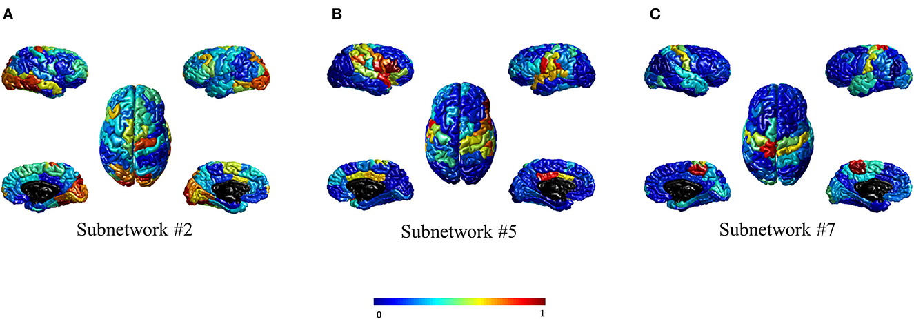
3.2. The most affected areas/links by SZ

For visualization purposes, the subnetworks were mapped onto the cortical surface by computing the nodal strength of each region concerning the ICA values. The nodal strength was computed as the summation of the absolute weights of all edges connected to that node. These nodal strength values were then normalized into the range [0–1] for each subnetwork. Figure 2 shows three significant subnetworks.

Figure 2. Three brain subnetworks significantly differentiated schizophrenia people from healthy controls. (A–C) show subnetworks #2, #5, and #7, respectively. The values are assigned to each region based on the normalized nodal strength. The maps are color-coded in which the larger value is shown in dark red and the smaller one in dark blue.

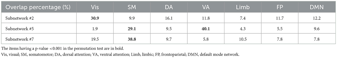
Figure 2 illustrates that high nodal strength values in subnetwork #2 are mostly observed in regions of the occipital cortex, while for subnetworks #5 and #7, regions in the parietal cortex, and the pre-, post-central gyrus are mostly allocated with high nodal strength, respectively. The visual inspection of subnetwork #2 in Figure 2A with the Yeo atlas (Yeo et al., 2011) indicated that the regions having high nodal strength mostly belong to the visual network. In addition, it seems that the regions in Figures 2B, C can be considered as part of ventral attention (VA) and somatomotor (SM) networks, respectively. This visual inspection was quantified through the computation of their overlap with the RSNs in the Yeo atlas (Yeo et al., 2011) using their nodal strengths. Table 3 represents the overlap percentage of these three subnetworks with the seven RSNs. The bolded values in Table 3 indicate the overlap percentages with p < 0.005 in the permutation test.

Table 3. Overlap percentage of subnetworks #2, #5, and #7 with the seven well-known RSNs.

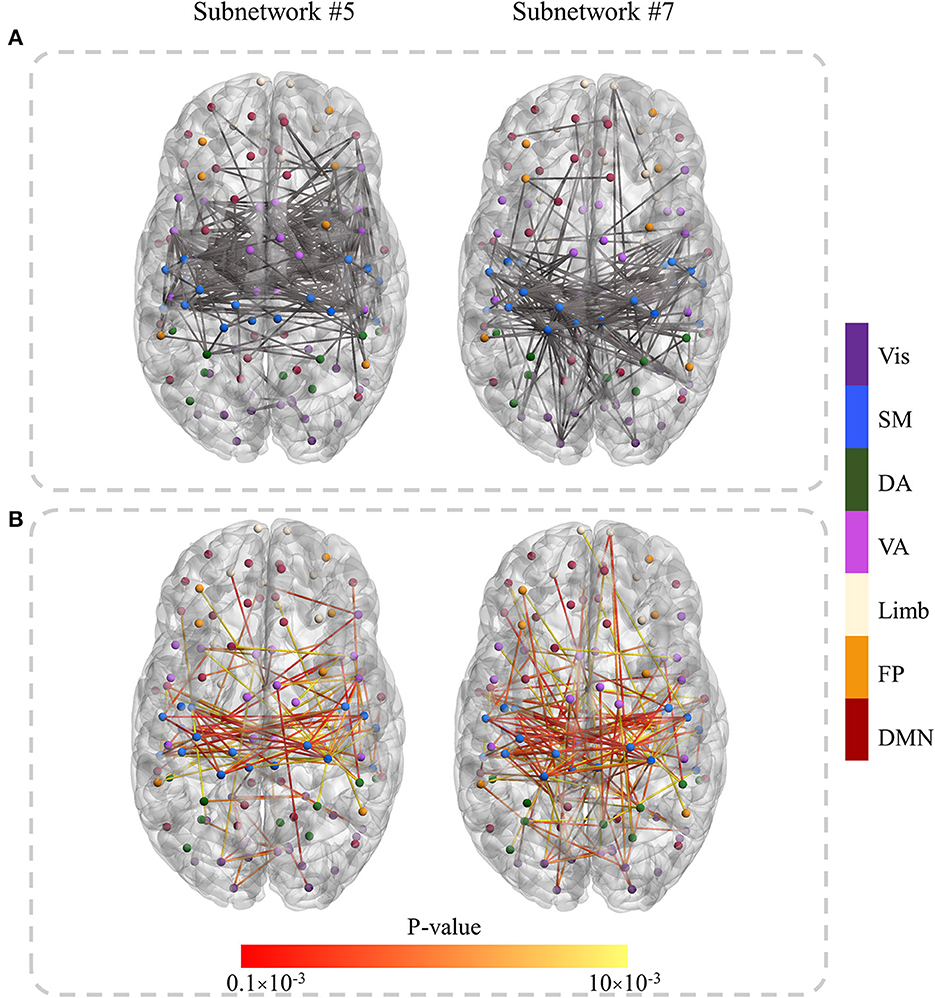
To further determine the discriminant connections of a subnetwork, we first selected connections with absolute ICA values >3.5. They are visualized in Figure 3A for the SZ-specific subnetworks (#5 and #7). Then for those selected connections, a t-test was performed over the original connectivity values between SZ and HC groups. Connections having p-value < 0.01 were visualized in Figure 3B as the most discriminant links (/connections) affected by SZ. It is evident from Figure 3 that the discriminant connections in subnetworks #5 and #7, in particular, link the SM and VA regions in two brain hemispheres.

Figure 3. The discriminant connections in subnetworks #5 and #7. (A) The connections with absolute ICA values above a threshold (3.5). (B) The most discriminant (p-value < 0.01) links that were obtained by applying the statistical t-test to the original functional connectivity of selected edges in (A). The node color determines the RSN they belong to. The lower p-value is shown in red in (B).

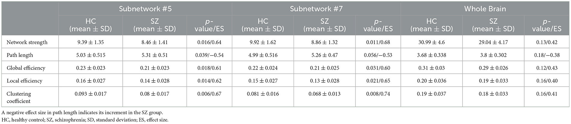
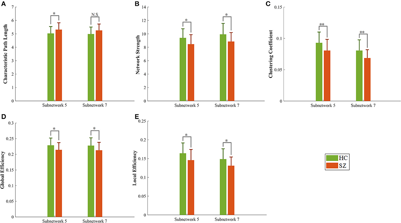
3.3. Graph parameters

There were no significant differences in characteristic path length, network strength, global efficiency, local efficiency, and clustering coefficient of the whole brain network between our limited number of participants in the HC and SZ groups (Table 4). Nevertheless, a significant difference in these five metrics was observed for two subnetworks #5 and #7 over the same dataset (Figure 4 and Table 4). The path length of the SZ group in subnetwork #7, however, was marginally significant. Moreover, the effect size of all metrics of #5 and #7 was >0.5, which implies their acceptable practical impact. All the measured graph metrics of the whole brain and the two subnetworks are given in Table 4. It should be mentioned that the p-value in other subnetworks was ≥0.1 for these graph parameters.

Table 4. Network topology metrics of two subnetworks, #5 and #7 as well as the whole brain.

Figure 4. Graph metrics of healthy (green bar) and schizophrenia (red bar) groups in two subnetworks #5 and #7. (A) Characteristic path length, (B) network strength, (C) clustering coefficient, (D, E) global and local efficiency. N.S, not significant, *p-value < 0.05, **p-value < 0.01.

4. Discussion

In the present study, the previously developed algorithm (Keyvanfard et al., 2020) was first modified and then applied to the population of 54 individuals including SZ and HC people. The algorithm output was the components related to the brain variations between individuals (Keyvanfard et al., 2020). The first eight components were considered for further analysis. Considering the selected edges in the subnetworks, three components indicated significant differences between the functional connectivity of SZ and HC groups.

4.1. Anatomical distribution of subnetworks

The second subnetwork had a significant and wide overlap (30.9%) with the visual network. Moreover, the statistical analysis of this subnetwork (Part A) indicated a significant difference between the HC and SZ. Therefore, it can be concluded that the visual network variations are somehow related to SZ. It is worth noting that the damaged and reduced functional connectivity of visual resting-state network in SZ people has been previously reported (van de Ven et al., 2017; Arkin et al., 2020; Keyvanfard et al., 2022; Wei et al., 2022). The prior independent reports have also demonstrated abnormalities in different levels of visual processing in individuals living with SZ (Butler et al., 2008; Green et al., 2011; King et al., 2017; Kogata and Iidaka, 2018; Adámek et al., 2022). Furthermore, the recent studies' results have discussed that the visual system has a possible key role in the development of SZ (Benson et al., 2012; Bolding et al., 2014; Morita et al., 2016; Császár et al., 2019).

Subnetwork #5 showed significant overlap (40%) with the ventral attention (VA) network. Its significant difference between the SZ and the control group indicated the functional connectivity of the VA network is disrupted in SZ. Deficits in attentional control are known as a main feature of SZ and a pivotal contributor to cognitive dysfunction (Luck and Gold, 2008; Nuechterlein et al., 2009; Orellana et al., 2012; Arkin et al., 2020). It has also been suggested that complex visual hallucinations reflect dysfunction within and between the attentional networks, leading to the inappropriate interpretation of ambiguous percepts (Shine et al., 2014). The VA network is closely associated with the so-called “salience network.” The salience network has been involved in the pathophysiology of SZ. Its dysfunction results in the incorrect assigning of salience, which can, in turn, lead to the key symptoms of SZ, including delusions (Palaniyappan and Liddle, 2012). Hypoconnectivity within the VA network has been previously reported in several studies (Yan et al., 2012; Wang et al., 2015; Dong et al., 2018;