A convenience sample of 32 healthy young participants was recruited for the study (16 males; age: 24.9 ± 3.6 years; body mass: 81.7 ± 9.7 kg; body height: 181.3 ± 7.5 cm; 16 females; age: 21.2 ± 3.5 years; body mass: 66.0 ± 7.8 kg; body height: 169.2 ± 5.7 cm). The required sample size was determined (α = 0.05; power = 0.80) based on previous studies that showed a significant moderate correlation between shear modulus, athletic performance and RFD (r =  ~ 0.4–0.5; Ando and Suzuki 2019; Ando et al. 2021a)) with 25 participants. Additional participants were recruited to prevent underpowering, as some studies with similar sample size (n = 24) failed to show a significant relationship between shear modulus and performance (Akkoc et al. 2018). The participants were all recreationally active in various sports (handball, soccer, volleyball and basketball), and reported that they were performing 3.6 ± 2.3 resistance training sessions per week in the last 6 months. The average body mass index was 23.9 ± 2.5 (24.6 ± 2.4 for males; 23.1 ± 2.3 for females). Exclusion criteria were any lower leg injuries in the past 6 months, pregnancy, any known neurological diseases, or any current musculoskeletal pain. Participants were thoroughly informed about the experimental protocol and written informed consent was required prior to commencing the study. The experiment was approved by National Medical Ethics Committee (approval no. 0120–99/2018/5) and was conducted in accordance with the latest revision of the Declaration of Helsinki.

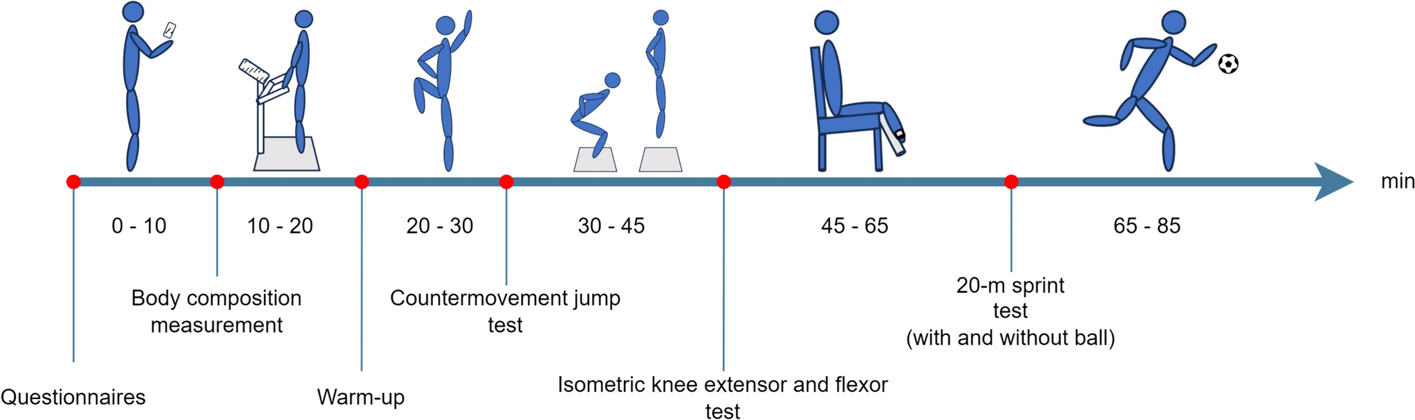
The participants were asked to refrain from any strenuous physical activity (i.e., resistance exercise and moderate-to-high intensity endurance activities) in 48 h before the measurement session. The experiment was conducted within a single session, lasting approximately 90 min. Upon arriving to the laboratory and signing the informed consent, the participants rested for 15 min in a prone position, after which the SWE measurements were taken. Then, the participants performed a warm-up consisting of 5 min of light-intensity running on a treadmill, 5 min of dynamic stretching (e.g., arm circles, leg swings, march and reach, trunk rotations) and a set of 5 bodyweight resistance exercises (10 squats, 5 push-ups, 5 lunges per leg, 5 submaximal countermovement jumps, 10 calf raises). The warm-up was designed to encompass the typical routines of recreational athletes, which ensures that the results of the study have the best validity in relation to typical sport conditions for these individuals. Then, the participant went on to perform (in that order) vertical jumping assessments, followed by isometric knee extension and ankle plantarflexion strength (peak torque) and explosive strength (RFD) assessments. Rest between measurement sections was 5 min. The order of the joints (knee, ankle) was randomized for each participant, while vertical jumping assessment always preceded the assessment of isometric strength and explosive strength. The experiment was carried out in an air-conditioned laboratory (23 ± 1 °C). The temperature was checked regularly using a Metrel® Multinorm (model MI 6201) with an microclimatic probe (model A1091).

In addition to examining the relationships between shear modulus, jump performance, and RFD on the whole sample, we also examined a potentially confounding effect of sex, age, body mass, and height. Namely, neuromuscular performance was expected to be higher in males than females (Bassett et al. 2020), while potential sex differences in muscle shear modulus are unclear at this point (Miyamoto et al. 2018; McPherson et al. 2020). Females could also have different shear modulus values due to a higher proportion of subcutaneous adipose tissue (Yoshitake et al. 2023).

Participants were instructed to lay prone and relax on a physical therapy table for 15 min prior to SWE measurements. As in previous studies using SWE (Morales-Artacho et al. 2017), this was done to minimize the possible confounding effects of prior activities (e.g., walking) on muscle shear modulus. The ankles were positioned over the edge of the table to ensure that the ankle was in neutral position. Then, we first obtained the shear modulus for medial (GM) and lateral (GL) head of the gastrocnemius, followed by the measurements for vastus medialis (VM) and vastus lateralis (VL). For the GM and GL assessments, the participant remained in the relaxed prone position and the probe was positioned on an imaginary line spanning from the heel to the medial and lateral condyles, respectively, on the most prominent aspect of the muscles. For VM and VL, the participants switched to supine position. For the VM, the probe was placed at distance 80% on the line between the anterior spina iliaca superior and the joint space in front of the anterior border of the medial collateral ligament. For VL, the probe was placed at 2/3 on the line from the anterior spina iliaca superior to the lateral side of the patella. For all muscles, the positions were carefully determined and the position marked with a non-permanent skin marker. For the VM and VL, we first performed the measurements at an extended knee position (knee angle 0°), followed by additional assessment at a flexed knee position (knee angle 90°). For the latter, the participant’s limb was moved to the appropriate position by the examiner to avoid muscle activation, and the knee angle was verified with a manual goniometer. Before SWE measurements, the B-mode ultrasound was used to ensure the parallel alignment with the direction of the muscle fascicles. A probe orientated in parallel to the muscle fascicles has been demonstrated to provide the most reliable and valid muscle stiffness assessment (Gennisson et al. 2010; Eby et al. 2013).

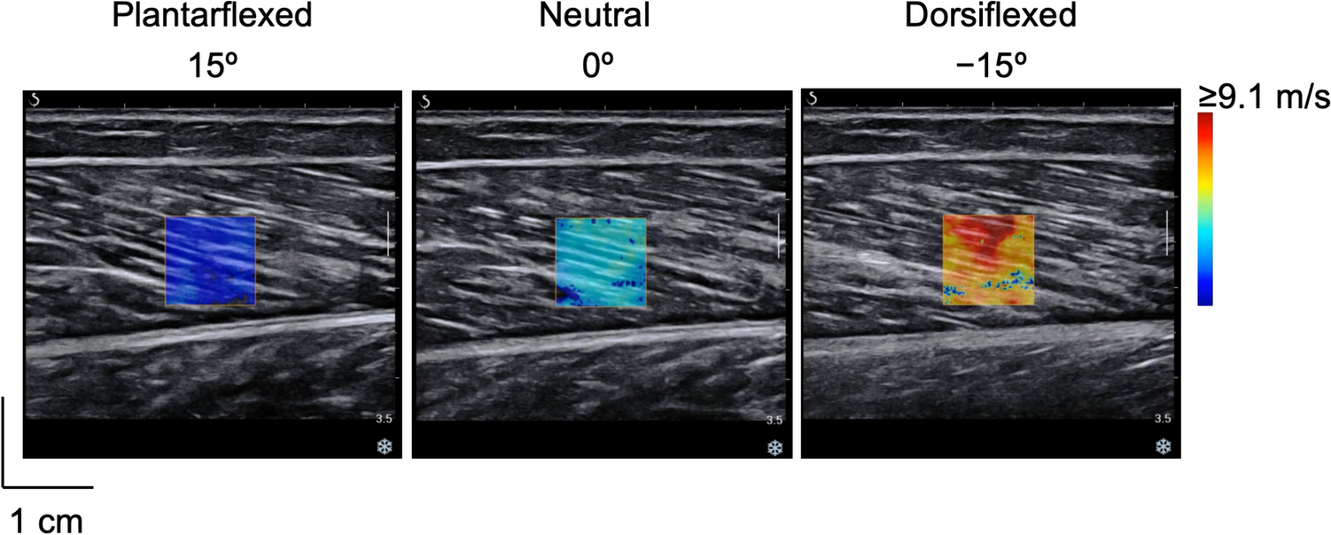
We used the Resona 7 ultrasound system (Mindray, Shenzhen, China), set to musculoskeletal mode, which assumes a tissue density of 1000 kg/m3. A 4-cm linear array probe (3–11 MHz; Model L11-3U, Mindray, Shenzhen, China) with a generous amount of water-soluble hypoallergenic ultrasound gel (AquaUltra Basic, Ultragel, Budapest, Hungary) was used. The region of interest was fixed at a square shape of 1 cm2. The depth of the region of interest was left to the choice of the examiner, with special care taken to only include muscle tissue. One measurement of the shear modulus assessment took about 8 s. The device takes 8 consecutive scans and displays the mean value. If the variability of the values within the 8 scans was above 15%, the measurement was repeated. In total, three measurements, with 1 min breaks in between, were performed and the mean value was taken for further analyses. Snapshots of ultrasound images are shown in Fig. 1.

Ultrasound image samples for lateral (A) and medial (B) head of the gastrocnemius, vastus lateralis (C) and vastus medialis (D) muscles. The white square represents the region of interests for shear modulus quantification

For each jump task (SJ and CMJ), the participants performed 2–3 attempts with submaximal effort, after which 3 repetitions were recorded for each jump in alternating order. Rest periods were set at 1 min between repetitions. For both jumps, the hands were placed on the hips throughout the entire trial. SJ was performed with the participant descending to the starting position which was achieved when the knee angle was at 90°. After stabilizing for 2–3 s, the jump was performed without countermovement. The examiner zoomed in and visually inspected the force–time trace on the computer and the trial was repeated in case any perceivable countermovement was detected (Pérez-Castilla et al. 2019; Suchomel et al. 2020; Janicijevic et al. 2022). For the CMJ, the participants were instructed to jump as high as and as fast as possible, using a countermovement (to the point where the knee angle was at 90°) and then immediately pushing off and extending forcefully through the hips, knees and ankles. Before each jump, participants were required to squat in a controlled manner until the desired position was reached to become familiarized with the 90° knee angle position, which was previously determined with a manual goniometer. In addition, an elastic band was positioned for each individual on the appropriate height to be in contact with participants’ buttocks when the desired angle was reached in SJ. For the CMJ, the elastic band was moved away from participants to avoid contact during the jump, and one examiner stood nearby the participant to visually control that the appropriate CMJ depth was reached (Janicijevic et al. 2022).

Ground reaction force data was captured with single force plate (Kistler, model 9260AA6, Winterthur, Switzerland). The signals were further automatically processed by the manufacturer’s software (MARS, Kistler, Winterthur, Switzerland) with a moving average filter (window: 5 ms). The vertical acceleration of the participant’s CoM was calculated via Newton’s second law of motion (F = m·a); subsequently, the acceleration was integrated to obtain vertical velocity using the trapezoid rule. Jump height was calculated from the takeoff velocity (TOV) as follows:

$$\mathrm\, \mathrm=\frac}^}$$

Were g is the acceleration of gravity (9.81 m∙s−2).

The best repetition (i.e., highest jump height) was taken for further analyses. CUR was calculated as follows: CUR = [CMJ-SJ]/SJ * 100%.

All isometric strength and RFD assessments were conducted using isometric dynamometers (S2P, Science to Practice, Ljubljana, Slovenia) with embedded force sensors (model 1-Z6FC3/200 kg) (Fig. 2). For the assessment of the ankle extension, the participant’s shins were tightly secured within the dynamometer frame, and the feet were placed on a rigid metal plate mounted on the force sensor. The axis of the dynamometer was carefully aligned with the medial malleolus and the ankle was in the neutral position (90°). The foot was tightly fixated against the plate with a strap. The knee and hip angles were set at 90° as well, which was achieved by adjusting the height and the depth of the dynamometer seat. For the assessment of the knee extension, the participants were seated in the dynamometer, tightly fixated across the pelvis and thighs, with the axis of the dynamometer aligned to the lateral femoral condyle. The knee angle was set to 60° (0° = full knee extension) and the hip was flexed at 90°. The instruction to the participants was to produce the force as “fast and as hard as possible”, and to maintain maximal exertion for ~ 3–4 s. The participants were instructed and constantly reminded to focus on emphasizing the explosive start (the fast part of the contraction). Three repetitions with 2 min breaks in between were performed. Loud verbal encouragement was provided at all times and the participants received real-time feedback on force trace on a computer screen.

Participant positioning for knee (left) and ankle (right) isometric strength assessments

The force signals were sampled at 1000 Hz and were further automatically processed in the manufacturer’s software (Analysis and Reporting Software, S2P, Ljubljana, Slovenia). A moving average filter (window: 5 ms) was applied, after which the RFD was calculated as Δ force /Δ time for 0–50, 0–100, 0–150 and 0–200 ms time windows. To ensure an accurate determination of force rise onset, we used custom-made software for semi-manual analysis (Maffiuletti et al. 2016). The instance of onset of torque rise was automatically detected by the software as the instant at which the baseline signal exceeded 3% of the peak torque. This was shown by a vertical marker placed on the torque-time trace. The examiner then zoomed in and moved the marker to more accurately determine the instant of force rise. Peak torque was determined as the mean value of the 1 s interval. For all of the outcome variables, the best repetition (i.e., highest value) was considered for the main statistical analyses (differences and correlations).

Statistical analyses were done with SPSS (version 25.0, SPSS Inc., Chicago, IL, USA). Descriptive statistics are reported as mean ± standard deviation. The normality of the data distribution was verified with a Shapiro–Wilk tests and visual inspection of Q-Q plots and histograms. The rep-by-rep reliability of outcome measures was assessed with the ICC (two-way random, absolute agreement model) and typical error, which was calculated as the standard deviation of the absolute differences between repetitions, divided by the square root of 2 (Hopkins 2000). Typical errors were expressed as % of the mean value (i.e., coefficient of variation; CV). The reliability according to ICC was interpreted as poor (< 0.5), moderate (0.5–0.75), good (0.75–0.9) and excellent (> 0.9) (Koo and Li 2016). The reliability according to CV was considered as excellent (< 5%), good (5–10%), acceptable (10–15%) and unacceptable (> 15%) (Shechtman 2013). Differences between males and females were examined with an independent-sample t-test. The associations between the outcome variables were assessed with Pearson’s product-moment correlations and interpreted as negligible (< 0.1), weak (0.1–0.39), moderate (0.4–0.69), strong (0.7–0.89) and very strong (> 0.9) (Schober and Schwarte 2018).We used a Benjamini–Hochberg method to control for the false discovery rate due to multiple correlations (Benjamini and Hochberg 1995). The threshold for statistical significance was set at α < 0.05.