1. Space, finally

Field potentials (FPs) reflect the operation of neuronal networks and as such, they are widely used to explore brain physiology and pathology. Amongst their advantages, FP waves can be recorded with high resolution, which makes them optimal signals to deal with the transient activation of neuronal populations. Moreover, their population nature provides an opportunity to monitor functional groups of neurons or cell assemblies (Fernández-Ruiz et al., 2012), these being viewed as the processing units of high-order structures (Abeles, 1991; Sakurai, 1998; Hanson et al., 2012; Papadimitriou et al., 2020). Given the primarily synaptic nature of FPs (Elul, 1971; Haberly and Shepherd, 1973), this paves the way to identify the anatomical correlates of any given activity.

Identifying the anatomical sources of brain potentials is not straightforward. We are used to visualizing FPs as pen traces that represent voltage fluctuations over time. However, brain potentials are space-varying three-dimensional signals that represent a mix of multiple sources (Supplementary Video 1), which has made their analysis difficult due to intrinsic restrictions and technical constraints. The poor access to the complex time-varying geometry of current sources has disengaged FP management from its causes, as manifested by the limited understanding of the factors that determine their amplitude and spatial extent. Decades of single-electrode recordings have led researchers to consider voltages at specific sites rather than fields in space, forging a widespread and erroneous view of the FPs generated by local neurons, even yielding the term local field potential (LFP) despite the fact that this does not make much sense in terms of physics. Indeed, electric fields extend beyond the populations that inject the current into the extracellular space and they may reach distant sensors while retaining significant amplitude (Lorente de Nó, 1947; Woodbury, 1960; Nunez and Srinivasan, 2006; Hales and Pockett, 2014). In the brain, such fields are commonly referred to as volume conducted potentials and they are often deemed negligible on the erroneous assumption that they decay dramatically as the distance from the neuronal source augments. Such an expectation is derived from the theoretical decay of the potentials from an ideal dipole (1/distance cubed). However, the complex filamentous structure of neurons prevents them from behaving as ideal dipoles, since the domains with net inward and outward currents (extracellular sinks and sources) have highly unequal spatial distribution and current density. In practice, each patch of membrane that experiences a current flow counts toward establishing extracellular potentials. Consequently, during population activation, the composite FP depends on the instantaneous value of current density and position of all active neural elements in 3D space, which leads to non-intuitive spatial distributions. Indeed, the activation of brain populations may or may not produce FPs (Lorente de Nó, 1947). As such, FPs may be negligible even at the center of the active population, or the amplitude may be even larger out of it. Both circumstances are incompatible with strict relationships with distance (Fernández-Ruiz et al., 2013). Evidence shows that FPs recorded in many brain structures get there by passive spread in the volume and actually arise in other regions (Carmichael et al., 2017; Lalla et al., 2017; Parabucki and Lampl, 2017; Bertone-Cueto et al., 2020). Meanwhile regions that produce significant FPs as the cortex and hippocampus also extend their potentials into each other’s domains (Torres et al., 2019), making FP waveforms multisource and site-dependent (Herreras et al., 2022). Significantly, electroencephalograms (EEGs) themselves are an entirely volume-conducted conglomerate of FPs (Nunez and Srinivasan, 2006).

The extension of FPs in space is generally poorly addressed in the literature. Some authors propose a generic spatial reach for any FPs, whereas others point to specific factors as the magnitude and size of the current source as the main determinants (Berens et al., 2008; Katzner et al., 2009; Liu et al., 2015). However, when referring to brain sources neither is correct, as it will become evident by the data reviewed below. The improvements in experimental capabilities in the last decade have finally allowed spatial information to be drawn from FP sources (e.g., multisite recordings: Benito et al., 2014; Herreras et al., 2015; Whitmore and Lin, 2016), which is rapidly changing the erroneous idea that they reflect nearby activities in individual populations. It has become evident that in addition to resolving a number of genuine questions about the FPs (Bédard et al., 2004; Reimann et al., 2013; Anastassiou and Koch, 2015; Herreras et al., 2022; Ness et al., 2022), some general concepts need to be fleshed out to bring them closer to the physical principles at play. As such, the recent boost to computational capabilities and the advances in simulation environments has made it possible to explicitly formulate a major problem, that of scaling micro to mesoscopic sources, which along with the dipolar nature of neuronal currents, will define the 3D geometry of FPs (Varona et al., 2000; López-Aguado et al., 2002; Fernández-Ruiz et al., 2013; Reimann et al., 2013; Torres et al., 2019; Herreras et al., 2022).

Until this century, the primary response to the problems caused by remote sources has been to try debugging FPs by eliminating distant contributions, such as for instance current-source density analysis (CSD: Mitzdorf, 1985). CSD helps determining the local or remote origin of FPs in the recorded sites (e.g., Carmichael et al., 2017). However, the CSD is unsuitable for spontaneous FPs by a number of reasons (Herreras et al., 2015), amongst which is the fact that they cannot separate the mixed potentials from strongly overlapping sources near the electrodes (LFPs) to recover reliable time courses for each of them (Martín-Vázquez et al., 2013).

Given the highly independent dynamics of different brain sources, the contribution of each to a specific recording site will depend on whether the associated FPs add or subtract from the others, and their relative weight there, establishing a kaleidoscopic of shifting contributions over time and space (Supplementary Video 1 and Figure 1). Conveniently, both the separation of sources and the determination of their local or remote origin can today be achieved advantageously by blind source separation techniques (see below) (Herreras et al., 2015; Whitmore and Lin, 2016; Torres et al., 2019). Before tackling this situation, it is important to understand how each source contributes to the amplitude of a FP and to its rate of decay. We have previously discussed a number of the misinterpretations of FP data that derive from simple recording settings and technical limitations (Herreras, 2016). Also, we offered guidelines to understand mesoscopic FPs from microscopic sources (Herreras et al., 2022). Here we will review recent multisite recordings and model multilevel data, discussing how they help the notions of volume conduction and our understanding of the spatial reach of FPs, more closely aligning these with the principles of physics. We focus on how variables related to single sources (e.g., size, shape, partial activation, uneven current density and dipolar nature) affect the amplitude and rate of decay of FPs. A number of experimental cases are reviewed illustrating how the particular cytoarchitecture of the activated region or structure affects the spatially uneven spread of their FPs and the implications of this for interpretation.

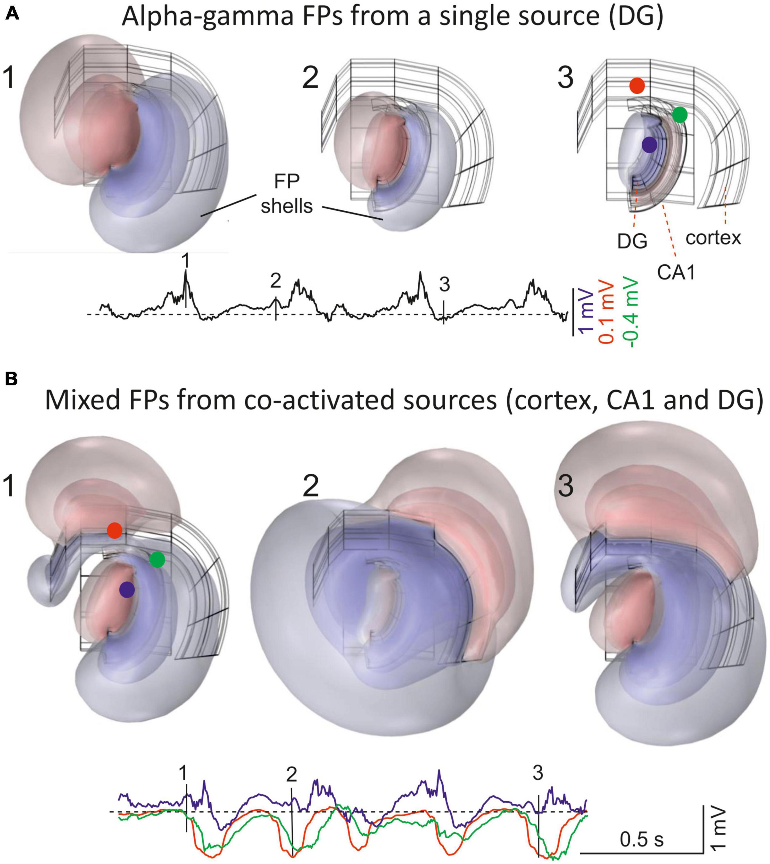
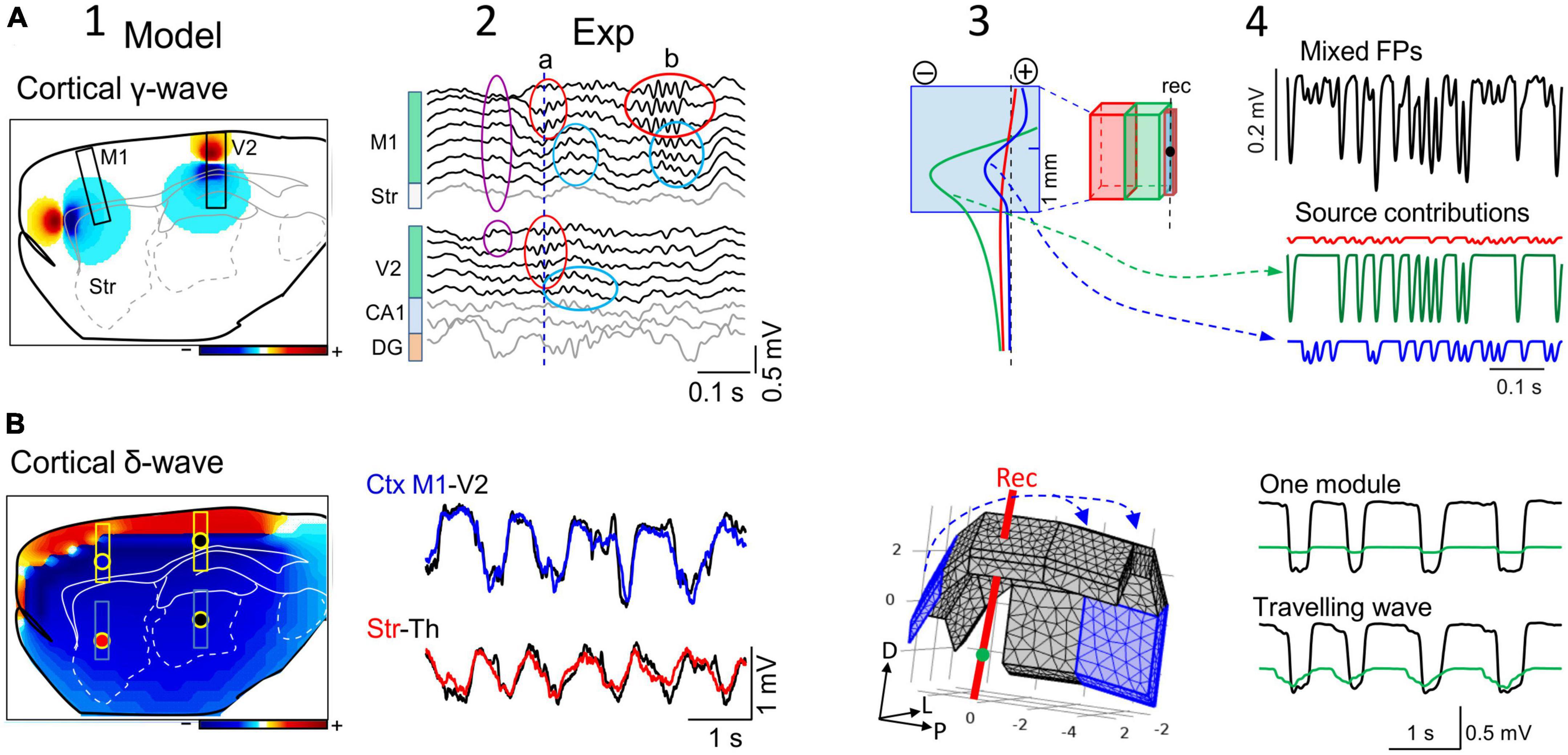
Figure 1. Field potentials (FPs) extend far from their population sources, invading other areas and mixing. (A) 1–3 are snapshots of the alpha-gamma activity generated in the Dentate Gyrus (DG). The instants chosen are indicated by vertical dashes in single site customary traces. The 3D structure of the sources is shown in the background in black. These were modeled as contiguous dipolar blocks of current (source and sink) with dimensions and spatial location roughly matching those in the Rat Brain Atlas by Patxinos and Watson (2006). Three pathway-specific sources of current were modeled, a synaptic input to middle dendrites of layer 5 pyramidal cells in the cortex (outer frame), an input to the st. lacunosum-moleculare of the CA1 pyramidal cells (intermediate), and the LPP input to Dentate Gyrus granule cells (inner frame). The colored concentric spheroids represent isopotential surfaces (blue and red shells of FP are negative and positive values, respectively). The lowest level plotted (outermost spheroid) is at ± 0.13 mV. These are from a point in the thalamus (blue) and two in the cortex (red and green) (note different scaling). (B) 1–3 snapshots during co-activation of multiple sources in different structures: alpha-gamma in the DG, slow waves in the cortex, and hippocampal theta rhythm in CA1. The model is based on finite-element methods (FEMs) using realistic dimensions, current densities and temporal dynamics (as in Torres et al., 2019). Note that FP shells at different instants maintain proportional amplitude across space when only one source is active (A), but not when multiple sources are co-activated (B). For a dynamic representation see Supplementary Video 1.

We first briefly introduce some general considerations that will help the spatial aspects of FPs.

1.1. How the properties of the medium affect FPs

The propagation and decay rate of electric fields in the brain follow principles that are common to any electromagnetic field. Hence, these features are determined by the characteristics of the source and the properties of the medium in which they propagate (resistive, diffusive, magnetic or inductive). The latter three were considered of little relevance by Lorente de Nó (1947) who proposed the quasi-stationary approach generally accepted as a reliable take on the volume-conductor theory in the brain (Woodbury, 1960; Plonsey, 1964; Rall, 1977; Nunez and Srinivasan, 2006). How the different electrical properties of tissues potentially influence the electrical fields within them has been considered on several occasions and some significant deviations of FP spread from expected in purely resistive media have been found (Elul, 1971; López-Aguado et al., 2001; Bédard et al., 2004, 2022; Holcman and Yuste, 2015; Savtchenko et al., 2017). However, it is widely accepted that the spatial extent of the FPs is not differentially affected within the most common frequency band of interest (0.1−200 Hz) (Nunez and Srinivasan, 2006; Ranta et al., 2017; Ness et al., 2022). Resistivity is not fully homogeneous in the brain and there are significant deviations from a uniform propagation of electric fields in regions where cellular elements of a particular geometry are grouped together (e.g., anisotropy in large fiber bundles), or where there are tissue heterogeneities (e.g., in layers with tight soma packing or near the ventricles: Li et al., 1968; Okada et al., 1994; López-Aguado et al., 2001; McCaan et al., 2019; Torres et al., 2019). These regions are important to bear in mind when tracking sources from recordings at remote sites, e.g., the EEG (Güllmar et al., 2015). Changes of tissue resistivity are also known to be produced during postnatal development, pathology or intense activity (Adey et al., 1966; Hoeltzell and Dykes, 1979; López-Aguado et al., 2001; Makarova et al., 2008), which should be used to correct for recorded FP values and predict their spatial reach. More important, brain sources have complex 3D geometry and are dipolar. It will be appreciated below that the impact of the source geometry on FP amplitude and spread exceeds by large the modulations derived from possible inaccurate appraisal of the mentioned properties of the volume conductor (see discussion in Herreras, 2016).

1.2. The pathway-specific nature of mesoscopic FPs: A conceptual leap

In contemporary literature, temporary characteristics of the FP are often used as the main identity card of a neuronal source (e.g., gamma or theta oscillations). The challenge, however, is to identify the anatomical substrates. It is already known that temporal patterns are not exclusive to a single source and that each source may express several patterns (Herreras, 2016; Herreras et al., 2022), further supporting the need for anatomical identification to avoid unfounded generalization of FP mechanisms in different structures.

If we were to find a structural unit of current that could serve as a canon for mesoscopic FPs, we would be in a position to predict the amplitude and spatial extent of the FPs generated by any given source through the use of anatomical information. At the microscopic level it was proposed that one or a small group of synapses (synaptic functional units) form extracellular dipoles from which FPs arise (Elul, 1971). However, the arborized structure of neurons distributes the current in such diverse ways that each synapse produces a unique extracellular 3D voltage shell (Rall, 1967; Behabadi and Mel, 2014; Toharia et al., 2016; Herreras et al., 2022). By the same token, individual neurons can be ruled out as elementary sources, since any single neuron can adopt innumerable geometries of dipolar currents when activated by different synapses, or by groups of them (Herreras et al., 2015, 2022).

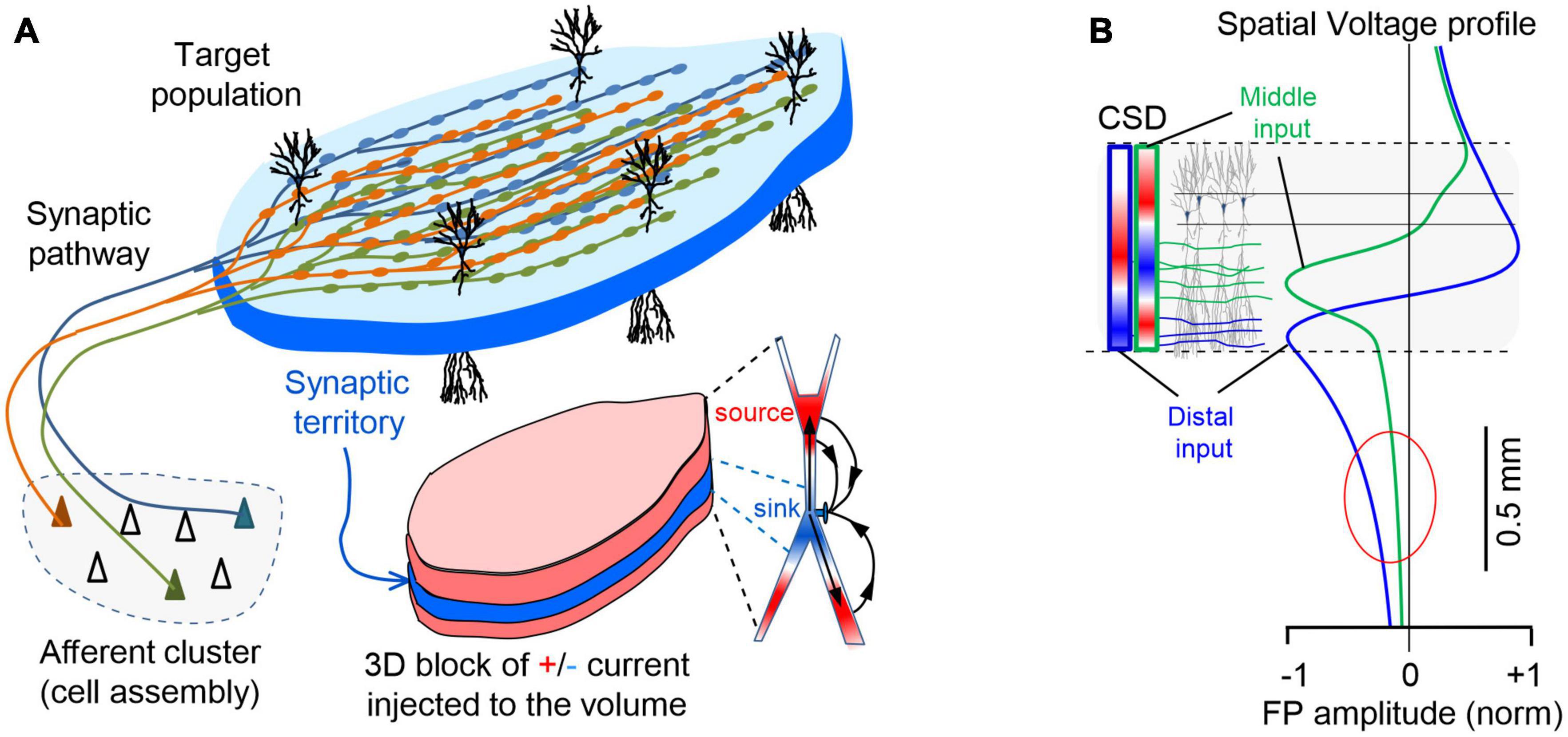
An invaluable reference at the mesoscopic level was finally attained through the application of spatial discrimination tools to high-density linear recordings in ordered structures (Korovaichuk et al., 2010; Makarov et al., 2010). Algorithms like independent component analysis (ICA, Bell and Sejnowski, 1995; Choi et al., 2005) can disentangle spatially coherent FP components that turn out to be pathway-specific (Fernández-Ruiz et al., 2012; Benito et al., 2014). Anatomically realistic computer models validated this approach (Makarova et al., 2011; Fernández-Ruiz et al., 2013), and led our team to propose a new anatomy-based concept of brain sources (Herreras et al., 2015). These were defined as the coherent extracellular currents produced by a specific neuron population upon synaptic input from a given pathway (Figure 2A). Consequently, the build-up and shaping of spontaneous FPs is similar to that of simple evoked potentials except that firing synchrony of the afferent population is less stringent (Fernández-Ruiz et al., 2012). This concept extends to the source/sink notion by Lorente de Nó (1947), which focused on cytoarchitecture of the population acting as source of current (neuron morphology and population arrangement), and adds an afferent pathway as a third element determining which part of the neurons/population will actually deliver the positive and negative currents to the surrounding volume. Indeed, grouped firing of neurons (cell assemblies) entails the synchronous activation of fibers within a pathway, which provides the necessary synchrony and spatial clustering of groups of synapses in the target population. The individual microscopic fields merge into coherent spatial blocks of FP activity, which in laminar populations peak in the synaptic territory (Benito et al., 2014). Naturally, since most pathways have a distinctive synaptic territory, the corresponding spatial blocks differ and cannot be used as canon. Note that asynchronous inputs in multiple pathways targeting the same population do not enable significant spatiotemporal summation of currents and in fact, they become unmeasurable (Elul, 1971; Łȩski et al., 2013). This concept helps visualize the FP source as a concrete 3D structure, closely matching the territory of a specific synaptic pathway from which FPs irradiate into the volume (see Supplementary Video 1). Also note that because of variable co-activation of multiple pathways one cannot expect a spatially stable structure of FP gradients in the volume and their disentanglement is necessary to access each one’s distribution and time-course (Herreras et al., 2015).

Figure 2. Spatial coherence of FPs is brought about by the pathway-specific nature of the sources. (A) The spatiotemporal clustering of currents required to raise a mesoscopic FP is provided by the synchronous firing of a cell assembly projecting onto an orderly population. The scheme illustrates a simple case corresponding to excitatory input from a neuron assembly to a target population with neurons arranged in palisade (e.g., the CA3-CA1 Schaffer pathway). Numerous buttons en passage ensure synchronous synaptic currents in the target population and the stratified organization of the synaptic territory can be perceived as an initial anatomical reference for source geometry (pad-like bluish block occupying a dendritic stratum). However, as the inward current at the synapses (sinks, in blue) travels inside neurons, it leaks out back into the volume (sources, in red) through adjacent membrane domains, jointly shaping a conglomerate of sheet-like stacked currents that cover the entire physical space occupied by the population. (B) Voltage profiles do not match CSD profiles. Computed voltage profiles for the activation of the Schaffer (green) and Perforant pathways (blue) that establish synaptic contacts in the middle and distal parts of the dendritic tree, respectively. The dashed lines represent the spatial boundaries of the source population within which the extracellular currents arise (colored bars on the left indicate the spatial distribution of currents for each pathway, i.e., the current source density: CSD) along the cell generators that produce the voltage profiles. Note the dipole or quadrupole (sandwich-like) configuration of the currents for inputs to distal or mid-dendritic portions of neurons, respectively. Distal inputs favor the extension of FPs away from the source population (oval).

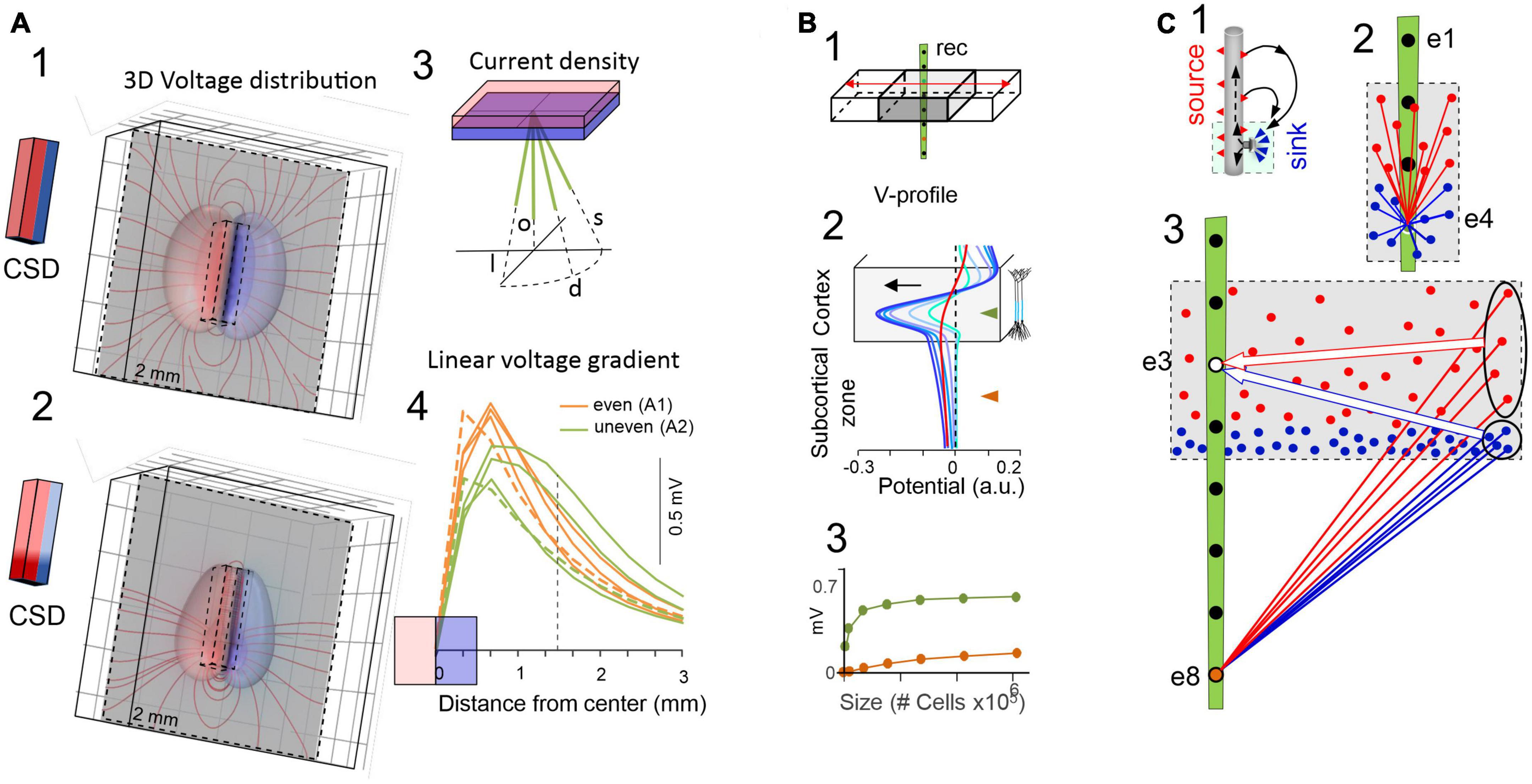
1.3. Spatial gradients of voltage give information on the location of sources and the spatial reach of the associated FPs

In examining the 3D voltage distribution of specific brain sources using realistic models, the spatial decay of FPs can be seen to vary in different directions, as reflected by the irregular spheroids formed by isopotential surfaces (Figure 1 and Supplementary Video 1). Sampling of these volumetric shells with linear arrays renders spatial voltage profiles that may vary along the source according to its geometry and the orientation of the array (Figure 3A). These profiles are important as they can also be achieved in experiments and provide a common tool to benchmarking the cellular and subcellular mechanisms. Thus, an ICA applied to multisite linear FPs returns a limited number of spatially coherent components, each characterized by a stable and unique spatial voltage profile (Makarov et al., 2010). Such single-source spatial profiles are time-invariant and they reflect the relative power along the recording array of the potentials elicited by an activated pathway (Figure 2B). Importantly, voltage profiles provide a stationary view of the reach of the FPs in the volume. For instance, accelerating curved spatial gradients indicate that the recording array is inside or close to the source, whereas non-zero, flat profiles correspond to remote sources. The latter phenomenon is explained by the small decay of potentials far from the source, maintaining similar amplitudes at all sites in high-density linear arrays. However, more complex spatial profiles can also be found, particularly for sources in curved structures (e.g., the hilus of the DG), and interpreting these requires anatomic guidance (Fernández-Ruiz et al., 2013).

Figure 3. The critical role of source geometry and current density in defining the rate of field potential decay. (A) Non-symmetrical dipolar sources produce FPs with different rates of decay. Panels (1,2) show the 3D computation of isopotential spheroids (only three levels are represented) generated by rectangular dipolar sources with the long side doubling the short one (4 mm × 2 mm × 0.5 mm). The lines of current are drawn on a plane perpendicular to the source. In panel (2) the source maintains the same overall geometry and total current density, but this is unevenly distributed. A few linear profiles of the voltage have been drawn (4) to better appreciate the different rates of decay. All plots depart from the center of the block as indicated in panel (3) and scan the volume orthogonal to the dipolar source (o), or they are tilted at identical angles to the long (l) or the short (s) sides, or in between (d). Profiles in orange and green correspond to 3D configurations in panels (1,2), respectively. It can be appreciated that the “mean” distance between the electrode and the source cannot be used to predict the amplitude and spatial reach of FPs. (B) Model analysis of the effect of increasing the size of a cortical module (0.5–6 mm) on the amplitude of the FPs recorded inside (gray) and outside subcortical sites (brown). Voltage profiles in panel (2) are colored from cyan to dark blue for enlarging cortical modules. The curved (in-source) and the flat portions (out-source) of the voltage profiles grow at different rates (3). Whereas the curved portion is mostly contributed by nearby neurons, the flat part can be said to be contributed by neurons at a distance from the recording tract. This distant contribution (red profile) can be computed by excluding neurons close to the electrode [neurons within 1 mm of the electrode were excluded in the red profile of panel (B) 2]. This is schematically explained in panel (C): Panel (1) is a scheme of the activation of an excitatory synapse and the resulting microscopic sinks and sources (blue and red arrowheads) on the outside, each of which raises a potential that integrates into recording sites weighted by distance. For small sources (2) the different distance of “point-like” sources or sinks determines the amplitude and polarity at electrodes inside the active population. For large sources (3) the distances of distant sources and sinks equalize at electrodes inside the population, largely neutralizing each other (large arrows), but less so for electrodes at a distance from the population (ovals). Although each “point-like” current has a small impact, the large numbers build significant potential over a distance. Thus, distance becomes irrelevant when many fields are combined and their joint geometry takes over [(B) reproduced with permission from Torres et al., 2019. (A) Computed with the same model].

One might expect that the spatial voltage profile would drop-off toward zero as it becomes distanced from the source. Such patterns have been found for several but not all hippocampal and cortical sources (Benito et al., 2014; Torres et al., 2019). In fact, spatial profiles often exhibit a curved segment and a flat tail with smaller amplitude that expands many millimeters from the source (Figure 3B), even covering the entire brain (e.g., slow cortical waves). The curved and the flat components can be experimentally detached from each other by the blockade of activity near the recording array. Detailed biophysical models indeed show that both spatial components belong to the same source (Torres et al., 2019), whereby the curved part is driven by the neurons closest to the recordings inside the source and the flat part by recordings outside and more distant (Figure 3C). In turn, the absence of decaying tails in a spatial voltage profile indicates that the generating sources do not extend significant potentials into other structures.

1.4. Dipolar neuronal currents make the mean distance to the source irrelevant as geometry prevails

There is a widespread notion that the distance from the source to a recording site determines the amplitude of the FP. However, when referring to brain sources, the generic use of the term distance is misleading since the sources are varied, heterogeneous and most importantly, dipolar. The mean distance from the source to a recording site does not explain why most brain structures do not contribute significant FPs despite their neurons being strongly activated. Similarly, it does not explain why different pathways elicit FPs in the same population that spread distinctly in the volume, or why a single pathway produces FPs with different rates of decay away from the same target (source) population.

Some cases have been illustrated in which the FP at a given distance from the center of the activated population acquires totally different values in different directions (Figure 3A). Rather than being caused by anisotropic media, this phenomenon is due to the 3D nature of the source and as such, the current density at all points within it needs be weighted at the chosen recording site to define the single-point voltage measurement. Indeed, some parts acts as a source (positive) and others act as sinks (negative), and the current density is likely to be non-uniform in each and with some parts closer than others (for an introduction to volume averaging of microscopic currents see Herreras et al., 2022). The mesoscopic dipoles remaining after cancellation of positive and negative miniature currents still retain a complex 3D geometry with uneven current densities (Figure 3C). Therefore, we should refer to favorable or unfavorable source geometries rather than to distance. This is not merely a semantic distinction, as the latter entails a simplification that supports what is often considered an insignificant impact of distant sources on FP recordings.

From the above considerations and given the complexity of brain sources, the amplitude of a FP at the origin does not determine how far it reaches. As such, rather than the peak magnitude of a current it is the overall spatial distribution and density of its sources and sinks that defines the rate of spatial decay of the potential. In some cases, this will be determined by the extension (size) of the activated population (Figure 3B) and/or the arrangement of neurons in space, whereas the location of the inputs may be the primary factor in other cases (Figure 2B). Thus, inputs to distal or middle portions of a dendritic tree produce far-reaching and mostly localized FPs, respectively, consistent with the overall dipolar or quadrupole configuration of the unbalanced electric sources and sinks in the volume (Herreras, 2016). This is relevant to identify which pathways produce FPs in one structure that will be exported to others. For instance, the lateral perforant pathway (LPP) input to distal dendrites of granule cells (distal input ≈ dipolar configuration) provokes potentials that reach the adjacent CA1 field and even the cortex, where they mix with FPs from local sources. By contrast, those FPs associated with activation of the medial perforant pathway (MPP) or Schaffer fibers (middle input ≈ quadrupole configuration) remain circumscribed to the Dentate Gyrus (DG) or the CA1, respectively, (Fernández-Ruiz et al., 2013; Benito et al., 2014). These geometrical constraints explain why hippocampal alpha waves may penetrate far into the cortex and other brain regions, whereas hippocampal sharp waves or gamma waves have a more limited spatial spread (Torres et al., 2019).

2. Local vs. volume-conducted field potentials: An ill-posed dilemma

At any instant, multiple sources are co-active in the brain. The global picture is that of a 3D space in which static regions act as variable sources of current and FPs are produced, exported and mixed in the volume conductor. The compound electrical field generated extends as a continuum through the volume of the brain, and it has space-varying amplitude according to each source’s location and rate of decay (Supplementary Video 1). The regions interposed between active sources still incorporate potentials from several others and these volume-conducted potentials also invade active sites, contaminating the FPs generated there. Consequently, whether a site hosts one, several or no sources, the FPs there will be a mixture. Indeed, the reputation of volume-conducted FPs as contaminants puts the spotlight on where we place the electrodes to minimize their impact, but this desirable goal is rarely pursued in practice, and may not be possible anyway (see below). Such contamination may confound measurement of waveform parameters (e.g., amplitude, phase, duration) and the frequency content of longer epochs (Herreras et al., 2022). Actions to minimize this problem typically involve multisite recording settings that enable nearby electrodes to be differentiated and off-line analytical removal through CSD analysis (Lorente de Nó, 1947; Leung, 1979; Mitzdorf, 1985). Modern approaches as spatial discrimination techniques (e.g., the ICA) do not remove any activity; rather they disentangle all sources and provide each one’s site of origin directly from the spatial profiles (Herreras et al., 2015).

Importantly, this “contaminating” idea by volume-conducted FPs has diverted attention away from the key fact that even after remote contributions are removed, the so-called local FPs (LFPs) are themselves mixtures, constituted of several close, or even overlapping sources. One might therefore consider that all FPs are mixtures of mutually contaminating sources, although this is an impractical notion and rather, we prefer to retain the more stringent terms of source co-activation and FP blending or mixture. Note that FPs recorded inside or outside of sources are not a strict parallel of local and volume-conducted potentials, since FPs are never local and all FPs are volume-conducted. Thus, we next discuss the distinguishing features of FPs in these two regions that help identify them in experimental recordings.

2.1. Field potentials originated in remote sources are ubiquitous and show distinguishing features

In all the brain structures explored to date through multisite recording and spatial discrimination techniques (e.g., the ICA), an FP component with non-zero flat spatial profile has been found (i.e., potentials that originate at sources remote to recording sites). By contrast, only a few structures yield FP components with curved spatial profiles (nearby sources) (Herreras et al., 2015). The relative variance of remote contributions is rarely below 5−10%, and it climbs to 100% in structures whose cytoarchitecture is not geometrically fit to generate mesoscopic sources of current (Martín-Vázquez et al., 2016). To gain an idea of how much voltage is introduced by sources beyond the recording position, it is helpful to compare differential (bipolar) to monopolar (grounded) recordings (Elul, 1962). The former typically show FPs about 10 times smaller than the latter (Gómez-Galán et al., 2012) and thus, most of the activity captured in FPs is remote rather than local. Several experimental studies indicate that FP activity originates from neurons circumscribed to a radius of a few hundred microns (Katzner et al., 2009; Liu et al., 2015). Actually, the rate of decay is specific to each source and cannot be generalized (e.g., Figures 2B, 3A). As a case in point, recent quantitative studies found that hippocampal theta and gamma rhythms in the rat brain may extend millimeters away from their sources, and these potentials have a large enough amplitude at distant sites to supersede local activity (e.g., the visual cortex: Torres et al., 2019). Other structures display FPs that are almost completely of a remote origin, such as in the striatum, the lateral septum and the habenula (Martín-Vázquez et al., 2016; Lalla et al., 2017; Bertone-Cueto et al., 2020). Detailed models confirmed that multipolar neuron morphology and/or the scattered arrangement of neurons in these structures does not favor the build-up of extracellular current sources and sinks, and hence FPs, as originally proposed by Lorente de Nó (1947). Recordings at different sites within structures with such unfavorable anatomical elements exhibit nearly identical FP fluctuations, as there are no local contributions to establish any spatial voltage gradients. Such cases are well detected by the ICA technique, which will only return components with flat spatial voltage profiles, i.e., all activity is volume driven from remote sites (Martín-Vázquez et al., 2016).

It then appears that so-called volume-conducted potentials are rather ubiquitous, and that they are likely to contribute to the waveform parameters of individual waves and the frequency content of long epochs anywhere (Herreras et al., 2022). As such, these potentials will introduce unknown error in quantitative studies that address functional connectivity using single electrodes. It should be noted that remote sources cause self-coherence when FPs are recorded in different structures (Florian et al., 1998; Torres et al., 2019).

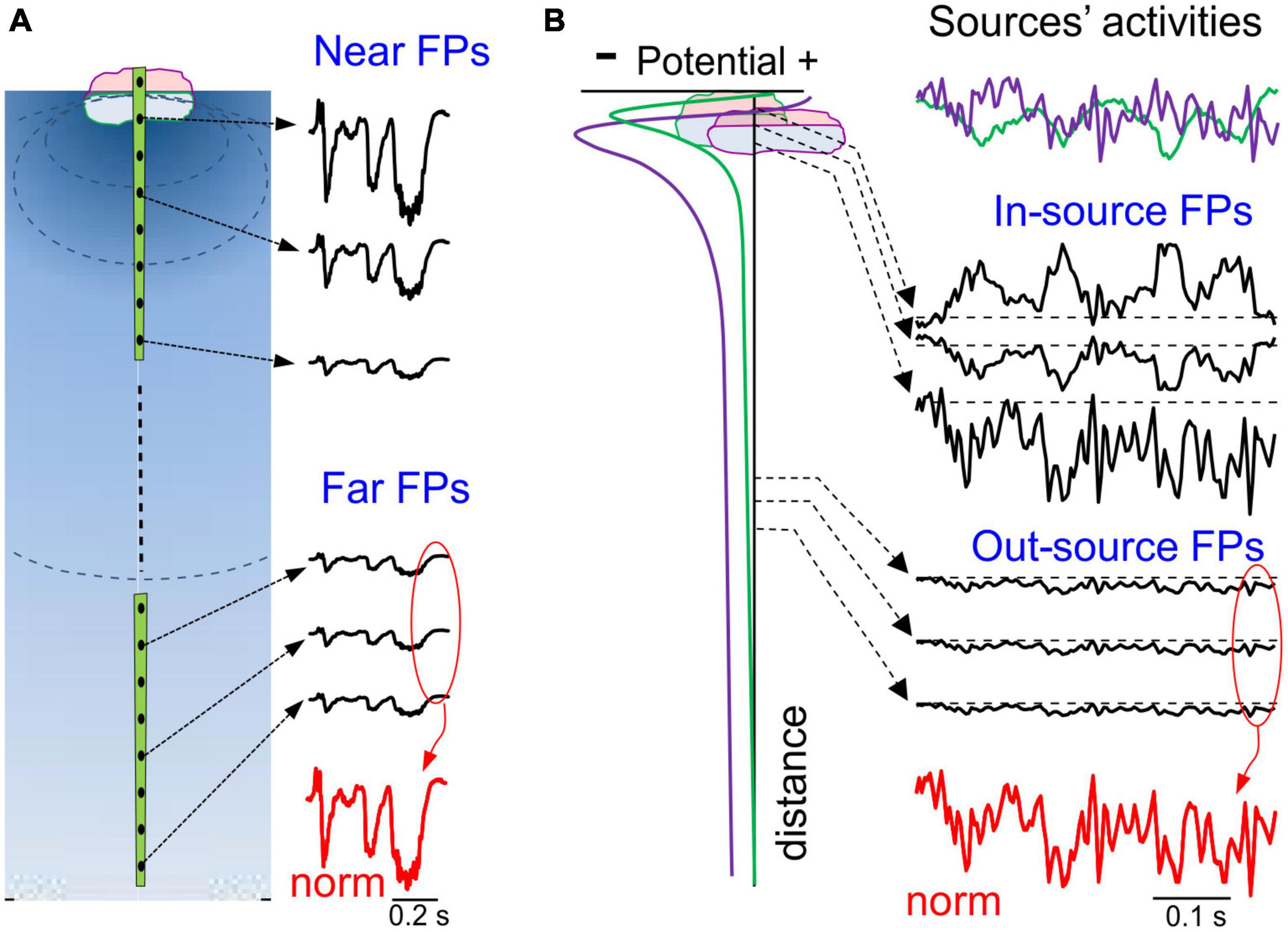
Since distant co-active sources contribute to remotely generated potentials, the time course of each cannot be discerned. In this sense, such potentials are as poorly defined as raw FPs or scalp EEGs, and they do not help discriminate whether they originated from one or many sources (Figure 4, red tracings). For instance, the FPs recorded in the lateral septum of anesthetized rats turned out to be entirely made up of remote contributions, and with temporal features reminiscent of both cortical and hippocampal sources (Martín-Vázquez et al., 2016). Also, FPs recorded in the striatum are entirely of a remote origin and they are a mixture of slow waves volume-conducted from the cortex, on top of which occasional bouts of alpha waves arise that can be traced to the hippocampus (Lalla et al., 2017; Torres et al., 2019). Identifying the structure of origin of remotely generated FPs is not trivial, although placing the test electrodes in the suspected sites, or even better, actively exploring the volume with moving multisite arrays may help.

Figure 4. Spatial and temporal ambiguities of potentials generated by local and remote sources. (A) Potentials decay fast close to the source and slowly away from it, a feature that is used as an arbitrary segmentation of the volume to circumscribe “local” and remote FPs. FPs elicited by a single source have an identical time course throughout the volume (normalized at the bottom in red), only varying in amplitude or polarity at different sites. (B) A case of two overlapping sources in the same structure (two synaptic pathways): left column, spatial voltage profiles; right column (from top to bottom), color coded activities of the two sources (top); in black, mixed FPs at different distances; at the bottom, normalized potentials of distant sites. Note that close to the sources the time course is strongly site-dependent, whereas at positions further away time features are invariant and exhibit blended time marks.

A distinct form of FP contamination, which also enters all recording sites in high density arrays with similar power, occurs when the reference electrode is placed at sites that pick up FPs, but this has no direct relation to volume conduction (Fein et al., 1988).

2.2. Features of not so local LFPs

Several pathways commonly converge on a given neuronal population and unless the synaptic territories match tightly, each pathway sets distinct zones of positive and negative current, i.e., the geometry of the respective dipolar sources differs even when arising from the same population of neurons. All regularly arranged structures so far explored through spatial discrimination techniques reveal multiple overlapping FP sources with distinct profiles along the somatodendritic axis of source neurons, which includes the cortex and hippocampus of rodents, and the lateral geniculate nucleus of monkeys (Benito et al., 2014, 2016; Makarova et al., 2014; Torres et al., 2019). Moreover, unpublished data from our lab includes the superior colliculus and the olfactory bulb of rodents in this category.

From a practical point of view, since each afferent pathway has its own dynamics, merging associated potentials into FPs diffuses the individual temporal patterns and hence, the waveform parameters become unreliable (see Figure 4 for an illustration of some aspects of this problem) (Martín-Vázquez et al., 2016). Steep gradients within the source population that decay outwardly in a pathway-specific manner are an important characteristic of FP mixing. In some regions of the brain, particularly in layered structures, each source’s relative contribution may vary considerably when the recording position is displaced only a small distance due to the strong stratification of the synaptic pathways. Hence, the temporal fluctuations in the mixed FP reflect the markedly different proportions of each pathway at different sites. In the hippocampus, spontaneous FPs may display large differences at sites as close as 100 microns (Benito et al., 2014) and in this regard, visual inspection of multisite linear recordings is sufficient to reveal smooth or strong spatial gradients. Spatial breakpoints can even be seen in recordings only 50 μm apart through the abrupt differences in the respective temporal features. These sites are generally associated with anatomic boundaries, such as the limits of two neuron populations, cell body layers or the demarcation of synaptic territories, which can help identify and/or localize the sources. As the distance to the sources increases, the spatial voltage gradients smooth out and flatten, such that their relative contribution stabilizes (Figure 4B).

As noted above, brain sources are not static entities and the volatile activation of synaptic pathways means that the spatial reach of FPs varies continuously. As such, a given recording period will contain remote and nearby sources that contribute to a varying degree over time. For instance, the amplitude (voltage) of any FP motif may vary with: (a) the proportion of neurons in a population activated that occupy stable spatial boundaries (fixed geometry); or (b) by additional recruitment of active neurons at more distant sites (varying geometry). In the latter case, since an electrode cannot provide information on the variations in the source, one may erroneously interpret a change in waveform parameters as reflecting the activation of different populations of neurons. In large structures, the extra voltage contributed by distant portions should be considered sensu stricto a remote contribution (“self-contamination”). The only way to overcome this uncertainty is by simultaneously recording from different parts of the same anatomical source.

3. The variable reach of field potentials from extended sources

Let us now review the experimental and modeling data that indicates how source geometry influences the amplitude and spatial extent of FPs originating in brain structures that are more favorable to FP build-up, such as the cortex and hippocampus. Orderly structures like these promote a segregation of the sources and sinks within their volume during the coherent synaptic activation of neurons, which is due to reduced cancellation among their neuron units. They are also optimally suited to spatial discrimination techniques that can reveal their multiple and often overlapping FP sources or generators. The voltage profiles obtained through these techniques reflect the spatial distribution of the FPs and offer a means to further investigate the relevant anatomo-functional mechanisms by matching them to those obtained in large-scale studies of anatomically realistic models. In this sense, a number of biophysical models have been deployed with sufficient anatomical and functional variables to provide time-varying FP gradients in 3D. These spatial gradients can be compared to experimental ones and they help identify the anatomical elements that produce them. Finite element methods (FEMs) and anatomically realistic (compartmental) neuron models can offer similar efficiency in the feed-forward reproduction of FPs in a volume conductor (Fernández-Ruiz et al., 2013; Torres et al., 2019; Ness et al., 2022), provided that the macroscopic sources used in the former accurately reproduce the spatial distribution and density of the currents (not the anatomy). Less realistic model approximations are not suitable as they cannot adequately discriminate suitable from unsuitable geometries of co-activated neurons and populations.

On the experimental side, some recording devices have been developed to gather 3D data (e.g., 3Dmatrix: van Daal et al., 2020), although they are still to be manufactured in a way that they can be scaled to obtain the entire 3D voltage shell of potentials elicited by brain sources that are too large or too small. By default, spatial samples of the voltage gradients (Figures 2B, 3A) can be obtained by exploring the volume with linear arrays (Benito et al., 2016; Ortuño et al., 2019; Orczyk et al., 2021). The instantaneous depth profiles of raw FPs vary continuously in concordance with the ongoing activation/deactivation of the sources. However, blind source separation techniques have proven efficient in separating these (Makarov et al., 2010; Herreras et al., 2015; López-Madrona and Canals, 2021).

The results reviewed pertain to geometrical conditions of the source that condition the interpretation of FP waves recorded inside the source volume (self-contamination), while also potentially highlighting the strong contribution and even dominance of FPs in other regions.

3.1. Field potentials from small cortical modules: Lateral cortico-cortical “contamination”

The neocortex is the largest structure in the mammalian brain and although it has a fairly well-maintained internal columnar organization, the area-specific afferent and associational circuitry establishes strong regionalization that defines discrete functional and operation modules (Arcaro and Livingston, 2021). Thus, the cortex is typically activated in a patchy pattern that reflects processing demands in behaving animals (Frostig et al., 2008; Çelik et al., 2021). In this state, functional cortical areas appear as small modular sources that process specific sensory cues, or information from body parts or related to cognitive tasks (Figures 5A1, A2; Katzner et al., 2009; Liu et al., 2015; Rogers et al., 2019). Biophysical models have shown that the size of different cortical areas determines how far cortical FPs reach into adjacent cortical areas (Figures 5A3, A4; Torres et al., 2019). In anesthetized rodents, some but not all of the alpha and gamma cortical generators extend through limited portions of the cortex, and the associated FPs reach a little beyond the physical boundaries of the respective modules (Figure 5A2). That is, the pronounced rate of voltage decay away from the source minimizes cortico-cortical contamination between adjacent modules.

Figure 5. The reach of cortical FPs depends on the specific geometry of the sources. (A) Computational (1) and experimental findings (2) on the activation of small cortical modules (0.5 mm) of layer 5 pyramidal cells during gamma waves in two cortical areas (M1 and V2). The computation is performed over the entire hemisphere (3D) but only one sagittal cut is shown with contour plots of the potential at a chosen instant. Scale color bar: ± 0.15 mV. The boxes mark the sites where recording arrays were placed in experiments to capture laminar FPs in panel (2). The limited spatial extent of gamma bouts in experiments is noted by the lack of coherence between the waves in different areas (a) or the region-selective occurrence (b). Other gamma waves (purple oval) appear with invariant waveforms along the cortical width and even in the striatum, indicating an extracortical origin of a gamma source that extends into large brain areas. Panels (3,4) show a different computer analysis of cortical blocks with independent dynamics and different sizes. It can be appreciated how small cortical modules (in blue) can exhibit FPs dominated by nearby larger modules (cortico-cortical contamination). The black trace corresponds to the FP mixture in the small module and the colored traces are the input activities to each module. The voltage profiles (3) and the time course of mixed FPs (4) show the greater contribution of near modules in red and green than its own. (B) (1) Similar computer simulation as in (A) for slow cortical (delta) waves spanning large portions of the cortical mantle predict that it reaches all sites in the rat brain with large amplitude (Scale color bar: ± 0.6 mV), which is confirmed in experiments (2). Actually, the amplitude reduces only moderately in subcortical sites far from their origin (the recording sites are marked by colored dots in “1”). Panel (3) illustrates the 3D representation of about 2/3rds of the cortical mantle used for the computation. Assembled rectangular blocks of dipolar current were used (numbers are mm). The blue arrows mark the direction of the slow wave traveling across the cortical modules. Upper traces in panel (4) represent the activation of a single cortical block, and the lower traces depict computed potentials during sliding activation (100 ms delay between contiguous cortical blocks) of the entire cortex [the first and last block are marked in blue in panel (3)]. (Columns 1 and 2, and panels (A3,A4) are adapted from Torres et al., 2019).

Since the degree of contamination depends on the relative size of active modules, the smaller the cortical module the greater the contamination of its FPs by adjacent ones (Torres et al., 2019), even to the point that they may be overshadowed by this contamination (Figures 5A3, A4). This fact must be taken into consideration when studying receptive fields or exploring the relationship between cortical regions. Note that since cortical modules may be activated in different epochs, the ongoing changes in wave parameters can be attributed indistinctly to local changes of excitability or to sporadic lateral contamination from adjacent modules. For example, different thalamo-cortical tracts activate similar synaptic territories of homologous cells in different cortical areas (Figure 5A2; Haegens et al., 2015). When nearby cortical modules emit fast rhythmic activities at a similar frequency, it may be anticipated that the resulting time-related parameters of gamma waves will be severely distorted in the merged FPs unless they are in phase (Herreras et al., 2022). Therefore, determining the extension of the functional modules of interest and that of their neighbors is essential. Anatomo-functional studies have outlined a number of cortical areas in different species, although it remains unclear if each of these serves as an independent source of current during spontaneous activity. Biophysical feed-forward models of synthetic FPs show that spatial discrimination techniques would be very effective to untangle the contributions of nearby and remote sources (Figures 5A3, A4).

3.2. Lateral contamination of FPs between adjacent areas is source-specific

Electrophysiology experiments show that each cortical region harbors several co-localized FP generators with distinct layer profiles (Martín-Vázquez et al., 2018; Ortuño et al., 2019; Orczyk et al., 2021). Since the geometry of the sources is defined by the topology and extent of the coherent synaptic inputs, the FPs of each may have a distinct lateral extension (Benito et al., 2014). The degree of lateral contamination between adjacent cortical areas is not expected to be area-specific but rather, source-specific. That is, synaptic inputs to some neuron types in the columnar circuits produce FPs that may spread more laterally than others. A laminar-specific extension of FPs and interlaminar coupling of currents has been seen in the cortex (Xing et al., 2009; Sotero et al., 2015), which is best explained by source specific geometric features, such as: (1) the range of horizontal connectivity; (2) the degree of stratification of the different pathways; (3) the subcellular location on the target neurons; or (4) their axial or multipolar anatomy.

3.3. Coherence across the cortical mantle means cortical FPs can reach everywhere subcortically

During slow wave sleep or under deep anesthesia, large portions of the cortex display highly coherent activity (e.g., slow waves, delta waves or Up-Down states: Destexhe et al., 1999; Riedner et al., 2011; Sánchez-Vives et al., 2017). Macroscopically, slow cortical waves travel across the tissue and several may even co-exist in different sectors of the cortical mantle (Massimini et al., 2004; Bernardi et al., 2018). The mechanisms underlying the synchronous and sliding activation of such large numbers of contiguous neurons across the cortex have been studied intensely but are yet to be fully defined. Coherent activation makes the myriad of individual neuron sources behave as an oversized single current source whose overall geometry and density (CSD) determines its spatial reach. The resulting potentials have an impact on adjacent and distant cortical areas, increasing the proportion of remote sources that contribute to FPs even at very distant sites (red profile in Figure 2B). A distinctive feature of such FPs is that the chemical blockade of synaptic activity near the recordings will produce a mild reduction in the amplitude of the FPs, whereas they will disappear rapidly if they arose from small cortical modules (Torres et al., 2019).

The most noticeable impact occurs at subcortical sites. For example, 1−2 Hz (delta) cortical waves with only moderate amplitude decay (≈50%) can be recorded in the striatum, thalamus, hippocampus, and any other small nucleus down to the base of the brain (Figure 5B2), mixing with local waves. These findings comply with theoretical studies that long ago showed that FPs in curved structures spread preferentially toward the concave side (Woodbury, 1960). When recording from subcortical structures with single electrodes, the large amplitude of such remote slow waves (up to 0.4−0.5 mV in adult rats) might lead one to consider they are nearby, an error that can be avoided through careful exploration of the spatial voltage gradients.

3.4. The different reach of FPs from co-localized sources may be paradoxical due to competing geometry-based influences

The combination in a given area of several sources from different cell populations, or their origin in the same neuron population, does not mean their respective FPs will have the same rate of spatial decay and reach, as other geometric factors may be at play. For example, simultaneous recordings at separate cortical sites show different voltage fluctuations riding on top of the slow waves (Mollazadeh et al., 2011; Volgushev et al., 2011; Torres et al., 2019). During the active phase of slow waves some areas may display alpha-beta oscillations that are not appreciated in others, or bouts of gamma waves may appear in one or two different areas that may or may not be in phase (Figure 5A2). These more rapid activities belong to smaller cortical modules than those involved in slow wave production and they may therefore not spread far subcortically. That is, the large cortical area activated during a slow wave contains smaller areas that are apparently activated independently within its physical boundaries.

Numerous studies have shown that many types of neurons can sustain different firing regimes, based on alterations to the rate and/or correlation of synaptic inputs. Such different input patterns can readily appear in FP dynamics, which in monolayered structures like the hippocampus may be ascribed to a single cell type capable of generating significant FPs (Makarova et al., 2011). We previously addressed this capacity of individual neurons in biophysical models (Herreras et al., 2015) and we found it to be caused by the pathway specificity of the FP generators. In experiments, we found that the laminar coverage and spatial extent of a source is determined by the topology of the afferent pathway, which determines spatial modules of coherent activity (i.e., the geometry of the source (Benito et al., 2014). It follows that an individual neuron, which is a geometrically stable entity, can act as geometrically different sources, as many as it receives synaptic pathways. This can be considered a general principle that can also be applied to the cortex, although its multilayered structure complicates the identification of cell and input pathways to individual sources (Ortuño et al., 2019; Torres et al., 2019). The different extensions of the sources will have notable consequences on the reach of their respective FPs into subcortical sites (compare Figures 5A1, 5B1). For example, while extended sources can be expected to produce far-reaching FPs, this can be counteracted by the distribution of the pathway input responsible for it over the cell, or by the morphology of the source neuron itself (Herreras et al., 2015, 2022; Martín-Vázquez et al., 2016). For the time being, these effects remain in the theoretical realm, as the reach of small or area-specific cortical FPs has been poorly addressed in experiments.

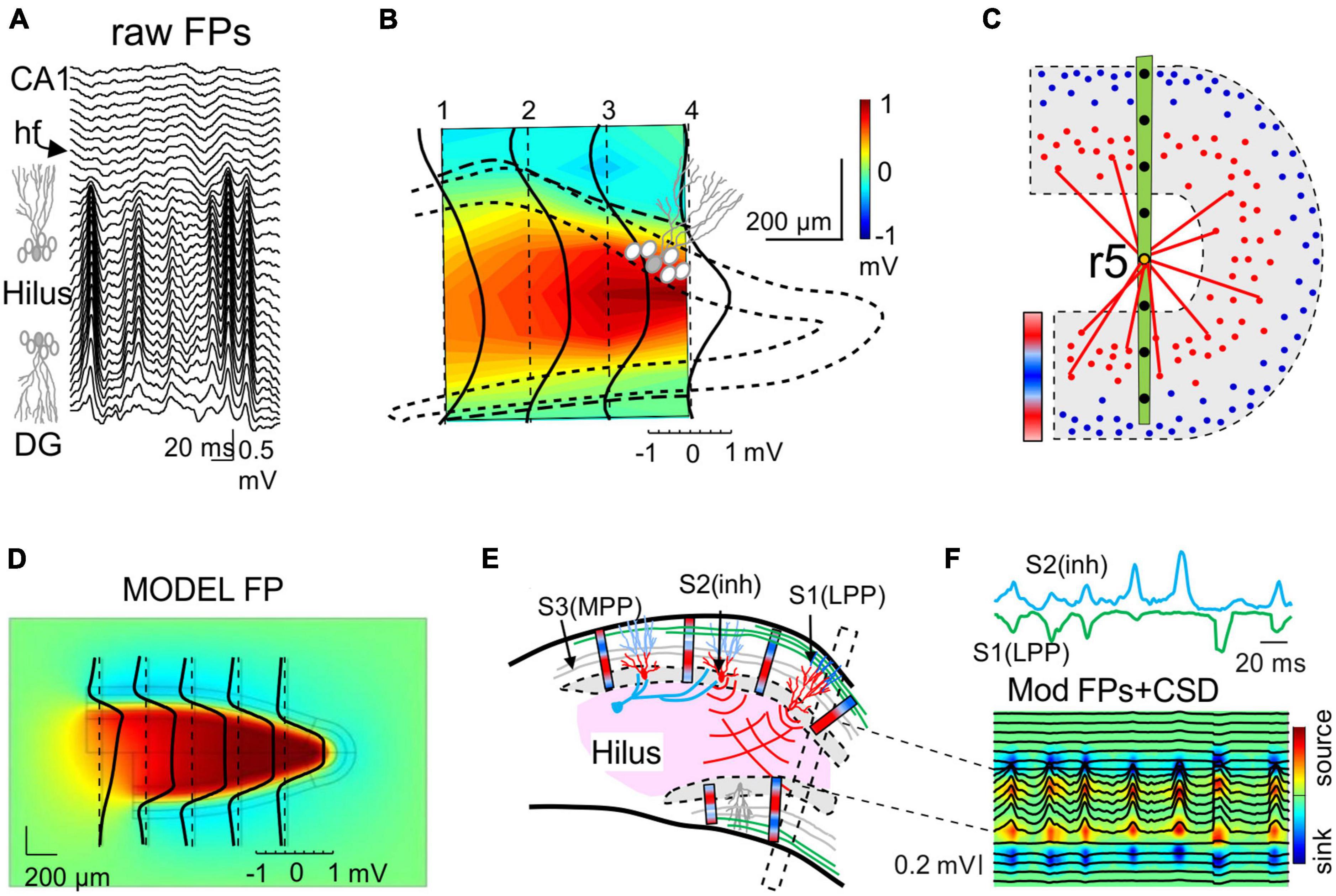
3.5. Giant FPs in the hilus are not local FPs

A remarkable case in which the architecture of a population defines the way FPs mix, and how far they reach, is the folding of the granule cell layer in the DG. Experimental examination of FPs in this curved region and realistic feed-forward computations have provided important lessons. First, the synaptic dendritic currents in the outer layers create dipolar curved sheets of current and a dramatic concentration of FPs in the interposed hilar region beyond the source granule cells, increasing up to 20 times in size of the value in the synaptic zone (Figures 6A, B, D; Fernández-Ruiz et al., 2013). This striking and yet paradigmatic case demonstrates that the amplitude of a FP is not sufficient to infer the location of the source of the current, and that anatomical knowledge of the candidate source is required.

Figure 6. Population curvatures promote greater FPs out of the physical space of the active neurons: the Hilus of the Dentate Gyrus. (A) Laminar recordings across the Dentate Gyrus (DG): synaptic inputs to granule cells (GCs) of the DG produce giant FPs in the Hilus between the folded layer of GCs. (B) Spatial display of the relative power of the medial perforant path (MPP)-specific FPs detached mathematically from other inputs. The dotted line outlines the GC body layer and the dashed line marks polarity reversal (zero value). The large positive potentials (yellow-red) in the Hilus (out of GC layers) outgrow the negative potentials in the synaptic layers 10–20-fold. The black lines are voltage profiles across different recording tracks. (C) Explanatory scheme of the potentials associated to an excitatory lateral perforant path (LPP) input in distal dendrites. Blue/red bar indicates the current density across GC layers: while the microsinks scatter in the outer dendritic layer (blue dots), the folding causes all the microsources (red dots) in both layers to cluster and approach the Hilus, fostering the combination of their potentials with respect to that of microsinks. The red lines indicate the similar proximity of the latter at the ends of both leafs to an electrode located in the middle of the Hilus (r5). These would be farther away if the GC layer were flat. Although the same can be said for microsources, the smaller average distance of the former has a greater impact. The bar represents the current density across the GC layers. (D) Model reconstruction of the relative power of FPs across a sagittal cut of the DG generated by synchronous MPP input to both layers (compare to B). (E) Scheme showing the cellular dipoles (blue/red bars) representing GCs receiving LPP input (S2) and somatic inhibition (S1). Note that the synaptic territories at both ends of GCs and opposing currents for somatic inhibition and dendritic excitation makes the respective dipoles orientate similarly. The dipoles in the upper and lower blades face each other and project with the same polarity (positive) toward the hilar region. The MPP input (S3, in gray) produces a quadrupole current distribution (not illustrated) that limits the spread of the potentials. The black box depicts the array recording area for traces illustrated in panel (F). (F) Model gamma oscillations elicited by a LPP excitatory input (S1, green) and soma inhibition (S2, cyan). The model was fed with source activities (colored traces) obtained from experiments to simulate FPs (black traces). The source/sink currents (CSD) generating the FPs are limited to GC layers, but they are absent in the Hilus. Note that all gamma waves recorded across the Hilus have similar polarity, whether contributed by one or the two inputs, and hence they could not reveal the synaptic origin [Panels (A,B,D) are taken from Fernández-Ruiz et al., 2013].

The second message drawn from the analysis of FPs in this curved region concerns the use of the polarity of waves as an indicator of the chemical nature of the synaptic pathway. It is widely believed that negative and positive waves reflect depolarizing and hyperpolarizing events, respectively. However, this viewpoint does not conform to the dipolar nature of neuronal currents that run across the membranes twice, forming inward-outward transmembrane loops. It also ignores the influence of remotely generated FPs on time-