1. Introduction

Glaucoma is known as a “silent thief of sight,” meaning that patients do not notice the health condition of their visual function until vision loss and even blindness occur (Abdull et al., 2016). According to the world health organization, the number of people with glaucoma worldwide in 2020 is 76 million, and the patient number would be increased to 95.4 million in 2030. As the population ages, the number with this condition will also increase substantially (Guedes, 2021). Glaucoma causes irreversible optic nerve vision damage. It is crucial to provide accurate early screening to diagnose patients in their early stages so that they can receive appropriate early treatment. Steady-state visual evoked potentials (SSVEPs), which refer to a stimulus-locked oscillatory response to periodic visual stimulation commonly exerted in the visual pathway of humans, can be used to evaluate the functional abnormality of the visual pathway that is essential for the complete transmission of visual information (Zhou et al., 2020). SSVEPs are always measured using electroencephalogram (EEG) measurement and have been widely used in the study of brain–computer interface (BCI). Because peripheral vision loss is a key diagnostic sign of glaucoma, patients cannot be evoked by certain repetitive stimuli with a constant frequency from vision loss regions (Khok et al., 2020). Therefore, stimuli with the corresponding frequency are not detected by the primary visual cortex. Thus, the SSVEPs-based BCI applications can be used in the early diagnosis of visual function detection for patients with glaucoma.

The effective analysis method for SSVEPs is critical in the accurate early diagnosis of glaucoma. SSVEPs are EEG activity with a spatial-spectral-temporal (SST) pattern. It is easy to understand that SSVEP signals, such as the EEG signal measured over time, could be analyzed using time series analysis methods. Brain functional connectivity (BFC) can be used to capture spatial patterns from multiple brain regions by analyzing the correlations between brain activities detected from different regions. The spectral pattern extraction method is the most popular method for analyzing the frequency characteristics of EEG signals. For instance, power spectra density–based analysis (PSDA) is a commonly used frequency detection method that can classify various harmonic frequencies from EEG signals (Zhang et al., 2020). In addition, canonical correlation analysis (CCA) (Zhuang et al., 2020) and other similar algorithms, such as multivariate synchronization index (MSI) (Qin et al., 2021) and correlated component analysis (COCA) (Zhang et al., 2019), are effective frequency detection algorithms based on the multivariate statistical analysis method. Although SST pattern extraction algorithms have demonstrated satisfactory results, most patterns or features extracted from raw EEG data require a manually predefined algorithm based on expert knowledge. The procedure of learning handcrafted features for SSVEP signals is not flexible and might limit the performance of these systems in brain activity analysis tasks.

In recent years, deep learning (DL) methods have achieved excellent performance in processing EEG-based brain activity analysis tasks (Li Z. et al., 2022; Schielke and Krekelberg, 2022). Currently, the mainstream technologies of using DL to process SSVEP signal could be divided into two aspects: convolutional neural network (CNN) based methods and transformer-based methods. For the CNN-based methods, Li et al. (2020) propose a CNN-based nonlinear model, i.e. convolutional correlation analysis (Conv-CA), to transform multiple channel EEGs into a single EEG signal and use a correlation layer to calculate correlation coefficients between the transformed single EEG signal and reference signals. Guney et al. (2021) propose a deep neural network architecture for identifying the target frequency of harmonics. Waytowich et al. (2018) design a compact convolutional neural network (Compact-CNN) for high-accuracy decoding of SSVEPs signal. For the transformer-based methods, Du et al. (2022) propose a transformer-based approach for the EEG person identification task that extracts features in the temporal and spatial domains using a self-attention mechanism. Chen et al. (2022) propose SSVEPformer, which is the first application of the transformer to the classification of SSVEP. Li X. et al. (2022) propose a temporal-frequency fusion transformer (TFF-Former) for zero-training decoding across two BCI tasks. The aforementioned studies demonstrate the competitive model performance of DL methods in performing SSVEPs-based BCI tasks. However, most existing DL efforts focused on applying existing techniques to the SSVEPs-based BCI task rather than proposing new ones specifically suited to the domain. Standard well-known network architectures are designed for data collected in natural scenes and do not consider the peculiarities of the SSVEP signals. Therefore, further research is required to understand how these architectures can be optimized for EEG-based brain activity data.

The main question is what is the specificity of the SSVEP signal analysis domain and how to use machine learning methods (particularly DL methods) to deal with the signal characteristics. Because the SSVEP signal is EEG-based brain activity, we can answer the question by analyzing the EEG characteristics in the brain activity analysis domain. Specifically, EEG characteristics are reflected in three aspects: temporal, regional, and synchronous characteristics. The temporal characteristics (e.g., mean duration, coverage, and frequency of occurrence) are easily traceable in standard EEG data and provide numerous sampling points in a short time (Zhang et al., 2021), thereby providing an efficient way to investigate trial-by-trial fluctuations of functional spontaneous activity. The regional characteristics refer to different brain regions that are linked to distinct EEG bands (Nentwich et al., 2020). The synchronous characteristics refer to the synchronous brain activity pattern over a functional network including several brain regions with similar spatial orientations (Raut et al., 2021). Traditionally, brain response to a flickering visual stimulation has been considered steady-state, in which the elicited effect is believed to be unchanging in time. In fact, the SSVEPs belongs to a signal with non-stationary nature, which indicates dynamical patterns and complex synchronization between EEG channels can be used to further understand brain mechanisms in cognitive and clinical neuroscience. For instance, Ibáñez-Soria et al. explored the dynamical character of the SSVEP response by proposing a novel non-stationary methodology for SSVEP detection, and found dynamical detection methodologies significantly improves classification in some stimulation frequencies (Ibáñez-Soria et al., 2019). Tsoneva et al. (2021) studied the mechanisms behind SSVEPs generation and propagation in time and space. They concluded that the SSVEP spatial properties appear sensitive to input frequency with higher stimulation frequencies showing a faster propagation speed. Thus, we hypothesize that a machine learning method that can capture the EEG characteristics in a unified manner can suit the SSVEPs-based BCI domain and improve the model performance in EEG-based brain activity analysis tasks.

In this study, we propose a transformer–based EEG analysis model known as the EEGformer (Vaswani et al., 2017) to capture the EEG characteristics in the SSVEPs-based BCI task. The EEGformer is an end-to-end DL model, processing SSVEP signals from the EEG to the prediction of the target frequency. The component modules of the EEG former are depicted as follows:

(1) Depth-wise convolution-based one-dimensional convolution neural network (1DCNN). The depth-wise convolution-based 1DCNN is first used to process the raw EEG input. Assuming the raw data is collected from C EEG channels, there are M depth-wise convolutional filters for generating M feature maps. Each convolutional filter is responsible for shifting across the raw data in an EEG-channel-wise manner and extracting convolutional features from the raw data of each EEG channel to form a feature map. Unlike other techniques that manually extract temporal or spectrum features based on the time course of the EEG signal, we use the depth-wise convolutional filter to extract the EEG features in a completely data–driven manner. Because the feature map is generated by the same depth-wise convolutional filter, each row of the feature map shares the same convolutional property. Follow-up convolutional layers are allocated with several depth-wise convolutional filters to enrich the convolutional features and deepen the 1DCNN network. A three-dimensional (3D) feature matrix is used to represent the output of the 1DCNN network. The x, y, and z dimensions of the 3D feature matrix represent temporal, spatial, and convolutional features, respectively.

(2) EEGformer encoder. This component module consists of three sub-modules: temporal, synchronous, and regional transformers, which are used in learning the temporal, synchronous, and regional characteristics, respectively. The core strategy of learning EEG characteristics by our model mainly include two steps: input tokens that serve as the basic elements of learning the temporal, synchronous, and regional characteristics are sliced from the 3D feature matrix along the temporal, convolutional, and spatial dimension, respectively. And then, self-attention mechanism is employed to measure the relationships between pairs of input tokens and give tokens more contextual information, yielding more powerful features for representing the EEG characteristics. The three components could be performed in a sequential computing order, allowing the encoder to learn the EEG characteristics in a unified manner.

(3) EEGformer decoder. This module contains three convolutional layers and one fully connected (FC) layer. The output of the last FC layer is fed to a softmax function which produces a distribution over several category labels. The categorical cross entropy combined with regularization was used as the loss function for training the entire EEGformer pipeline. The EEGformer decoder is used to deal with specific tasks, such as target frequency identification, emotion recognition, and depression discrimination. In addition to using a large benchmark database (BETA) (Liu et al., 2020) to validate the performance of the SSVEP-BCI application, we validate the model performance on two additional EEG datasets, one for emotion analysis using EEG signals [SJTU emotion EEG dataset (SEED)] (Duan et al., 2013; Zheng and Lu, 2015) and the other for a depressive EEG database (DepEEG) (Wan et al., 2020) obtained from our previous study, to support our hypothesis that highlights the significance of learning EEG characteristics in a unified manner for EEG-related data analysis tasks.

The main contributions of this study are as follows: (1) current mainstream DL models have superior ability in processing data collected in natural scenes and might not adept at dealing with SSVEP signals. To achieve a DL model that can be applied to the specificity of the SSVEP signal analysis domain and obtain better model performance in SSVEPs-based frequency recognition task, we propose a transformer–based EEG analysis model known as the EEGformer to capture the EEG characteristics in a unified manner. (2) To obtain a flexible method for addressing the SSVEPs-based frequency recognition and avoid the model performance limited by manual feature extraction, we adopt 1DCNN to automatically extract EEG-channel-wise features and fed them into the EEGformer. This operation transforms our method into a complete data–driven manner for mapping raw EEG signals into task decisions. (3) To ensure the effectiveness and generalization ability of the proposed model, we validate the performance of the EEGformer on three datasets for three different EEG-based data analysis tasks: target frequency identification, emotion recognition, and depression discrimination.

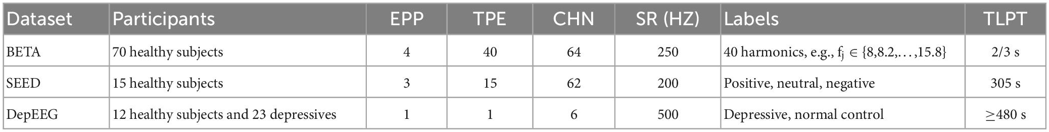
2. Materials and methods 2.1. Dataset preparation

Table 1 shows some detailed information about the three datasets (BETA, SEED, and DepEEG) that we used as benchmarks to validate the effectiveness of this study. The participants’ column in the table describes how many subjects joined in the corresponding data collection. The experiment per participant (EPP) column shows how many experiments were performed by each participant. The trails per experiment (TPE) column shows how many trails are executed in one experiment. The channel number (CHN) column shows the CHN of the EEG dataset. The sampling rate (SR) column shows the down-sampling rate of the EEG signal. The time length per trail (TLPT) column shows the time length of a single trail in seconds. The labels column shows the categorical emotion labels for the classification task and emotional intensity for the regression task. Specifically, for the target frequency identification task, we classified 40 categories of harmonic frequencies and the frequency range is 8–15.8 HZ with 0.2 HZ intervals. For the emotion recognition task, we used arousal, valence, and dominance rating scores as the dataset labels. For the depression discrimination task, we classified EEG samples from depressive or normal control.

Table 1. Detail information on the three datasets.

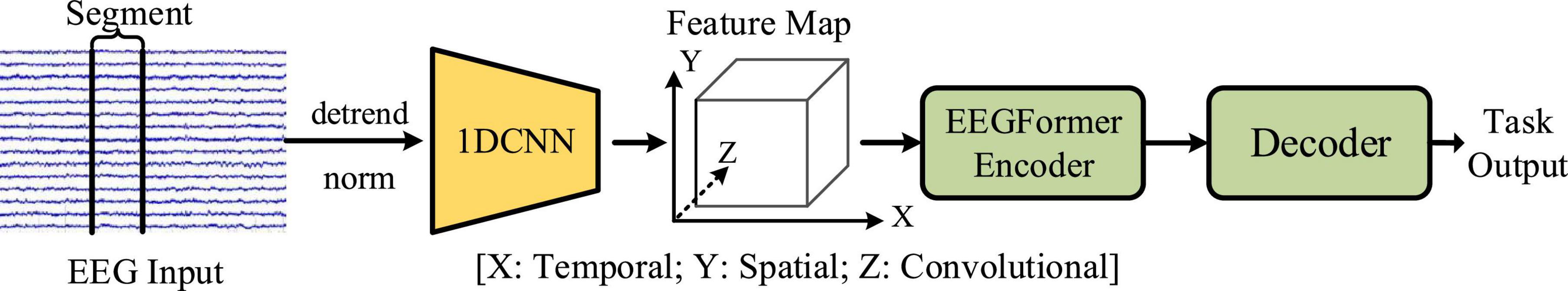
2.2. Pipeline of EEGformer–based brain activity analysis

Figure 1 shows the pipeline of EEGformer–based brain activity analysis. The core modules of the pipeline include 1DCNN, EEGformer encoder, and decoder. The input of the 1DCNN is an EEG segment represented using a two-dimensional (2D) matrix of size S × L, where S represents the number of EEG channels, and L represents the segment length. The EEG segment is de-trend and normalized before being fed into the 1DCNN module, and the normalized EEG segment is represented by x ∈ RS × L. The 1DCNN adopts multiple depth-wise convolutions to extract EEG-channel-wise features and generate 3D feature maps. It shifts across the data along the EEG channel dimension for each depth-wise convolution and generates a 2D feature matrix of size S × Lf, where Lf is the length of the extracted feature vector. The output of the 1DCNN module is a 3D feature matrix of size S × C × Le, where C is the number of depth-wise convolutional kernels used in the last layer of the 1DCNN module, Le is the features length outputted by the last layer of the 1DCNN module. More specifically, the 1DCNN is comprised of three depth-wise convolutional layers. Hence, we have the processing x → z1 → z2 → z3, where z1, z2, and z3 denote the outputs of the three layers. The size of the depth-wise convolutional filters used in the three layers is 1 × 10, valid padding mode is applied in the three layers and the stride of the filters is set to 1. The number of the depth-wise convolutional filter used in the three layers is set to 120, ensuring sufficient frequency features for learning the regional and synchronous characteristics. We used a 3D coordinate system to depict the axis meaning of the 3D feature matrix. The X, Y, and Z axes represent the temporal, spatial, and convolutional feature information contained in the 3D feature matrix, respectively. The output of the 1DCNN module is fed into the EEGformer encoder for encoding the EEG characteristics (regional, temporal, and synchronous characteristics) in a unified manner. The decoder is responsible for decoding the EEG characteristics and inferencing the results according to the specific task.

Figure 1. Pipeline of EEGformer for different tasks of brain activity analysis.

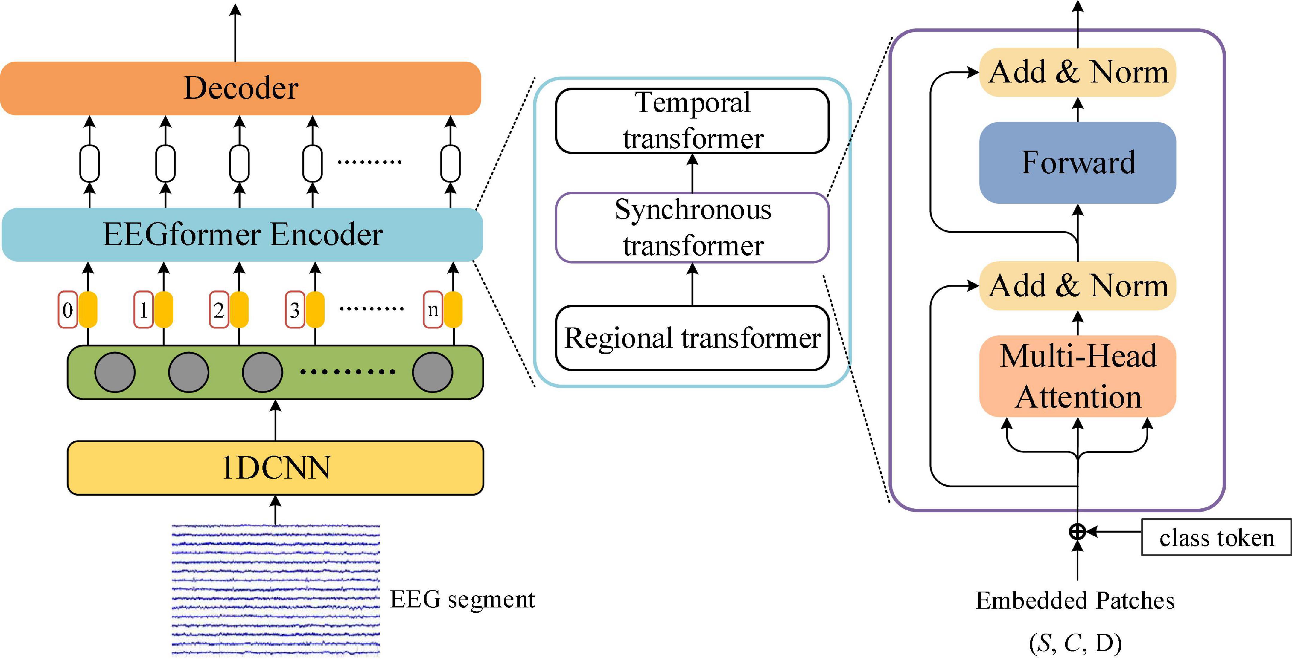
2.3. EEGformer encoder

The EEGformer encoder is used to provide a uniform feature refinement for the regional, temporal, and synchronous characteristics contained in the output of the 1DCNN module. Figure 2 illustrates the EEGformer architecture and shows that the EEGformer encoder uses a serial structure to sequentially refine the EEG characteristics. The temporal, regional, and synchronous characteristics are refined using temporal, regional, and synchronous transformers, respectively. The outputs of the 1DCNN are defined as z3 ∈ RS×C×Le and are represented using black circles in the green rectangle box.

Figure 2. Illustration of the EEGformer architecture.

The specific computing procedures of each transformer module are depicted as follows:

2.3.1. Regional transformer module

The input of the regional transformer module is represented by z3 ∈ RC×Le×S. The 3D matrix z3 is first segmented into S 2D submatrices along the spatial dimension. Each submatrix is represented by Xir⁢e⁢g∈RC×Le (i = 1,2,3,…,S). The input of the regional transformer module is represented by S black circles in the green rectangle box and each circle represents a submatrix. The vector X(i,c)r⁢e⁢g∈RLe is sequentially taken out from the Xir⁢e⁢g along the convolutional feature dimension and fed into the linear mapping module. According to the terminology used in the vision of transformer (ViT) studies, we defined the vector X(i,c)r⁢e⁢g as a patch of the regional transformer module. Each X(i,c)r⁢e⁢g is represented by a tiny yellow block in the Figure 2. The X(i,c)r⁢e⁢g is linearly mapped into a latent vector z(i,c)(r⁢e⁢g,0)∈RD using a learnable matrix M ∈ RD×Le:

z(i,c)(r⁢e⁢g,0)=M⁢X(i,c)r⁢e⁢g+e(i,c)p⁢o⁢s,(1)

where e(i,c)p⁢o⁢s∈RD denotes a positional embedding added to encode the position for each convolutional feature changing over time. The regional transformer module also consists of K ≥ 1 encoding blocks, each block contains two layers: a multi-head self-attention layer and a position-wise fully connected feed-forward network. The resulting z(i,c)(r⁢e⁢g,0) is defined as a token representing the inputs of each block, and the z(0,0)(r⁢e⁢g,0) indicates the classification token. The l-th block produces an encoded representation z(i,c)(r⁢e⁢g,l) for each token in the input sequence by incorporating the attention scores. Specifically, at each block l, three core vectors, including q(i,c)(l,a), k(i,c)(l,a), and v(i,c)(l,a) are computed from the representation z(i,c)(r⁢e⁢g,l-1) encoded by the preceding layer:

q(i,c)(l,a)=WQ(l,a)⁢L⁢N⁢(z(i,c)(r⁢e⁢g,l-1))∈RDh,(2)

k(i,c)(l,a)=WK(l,a)⁢L⁢N⁢(z(i,c)(r⁢e⁢g,l-1))∈RDh,(3)

v(i,c)(l,a)=WV(l,a)⁢L⁢N⁢(z(i,c)(r⁢e⁢g,l-1))∈RDh,(4)

where WQ(l,a), WK(l,a), and WV(l,a) are the matrixes of query, key, and value in the regional transformer module, respectively. LN() denotes the LayerNorm operation, and a ∈ is an index over the multi-head self-attention units. A is the number of units in a block. Dh is the quotient computed by D/A and denotes the dimension number of three vectors. The regional self-attention (RSA) scores for z(i,c)(r⁢e⁢g,l-1) in the a-th multi-head self-attention unit is given as follows:

α(i,c)(l,a)r⁢e⁢g=σ⁢(q(i,c)(l,a)Dh⋅[k(0,0)(l,a)⁢c=1,…,C])∈RC,(5)

where σ denotes the softmax activation function, and the symbol ⋅ denotes the dot product for computing the similarity between the query and key vectors. k(i,c)(l,a) and q(i,c)(l,a) represent the corresponding key and query vectors, respectively. The equation shows that the RSA scores are merely computed over convolutional features of single brain region. That is, the RSA can calculate the contribution of a changing mono-electrode convolutional feature to the final model decision at a specific EEG channel. An intermediate vector s(i,c)(l,a) for encoding z(i,c)(r⁢e⁢g,l-1) is given as follows:

s(i,c)(l,a)=α(i,0)(l,a)⁢v(i,0)(l,a)+∑j=1Cα(i,j)(l,a)⁢v(i,j)(l,a)∈RDh.(6)

The encoded feature z(i)(r⁢e⁢g,l)∈RC×D by the l-th block is computed by first concatenating the intermediate vectors from all heads, and the vector concatenation is projected by matrix WO ∈ RD×L, where L is equal to A=Dh. z(i)(reg,l)′ is the residual connection result of the projection of the intermediate vectors and the z(i)(r⁢e⁢g,l-1) encoded by the preceding block. Finally, the z(i)(reg,l)′ normalized by LN() is passed through a multilayer perceptron (MLP) using the residual connection. The output of the regional transformer is represented by z4 ∈ RS×C×D.

2.3.2. Synchronous transformer module

The input of the synchronous transformer module is represented by z4 ∈ RS×Le×C. The 3D matrix z4 is first segmented into C 2D submatrices along the convolutional feature dimension. Each submatrix is represented by Xis⁢y⁢n∈RS×D (i = 1,2,3,…,C). The vector X(i,s)s⁢y⁢n∈RD is sequentially taken out from the Xis⁢y⁢n along the spatial dimension and fed into the linear mapping module. The X(i,s)s⁢y⁢n is defined as a patch and is linearly mapped into a latent vector z(i,s)(s⁢y⁢n,0)∈RD using a learnable matrix M ∈ RD×D:

z(i,s)(s⁢y⁢n,0)=M⁢X(i,s)s⁢y⁢n+e(i,s)p⁢o⁢s,(7)

where e(i,s)p⁢o⁢s∈RD denotes a positional embedding added to encode the spatial position for each EEG channel changing over time. The synchronous transformer also consists of K ≥ 1 encoding blocks, and each block contains two layers: a multi-head self-attention layer and a position-wise fully connected feed-forward network. The resulting z(i,s)(s⁢y⁢n,0) is defined as a token representing the inputs of each block, and the z(0,0)(s⁢y⁢n,0) indicates the classification token. The l-th block produces an encoded representation z(i,s)(s⁢y⁢n,l) for each token in the input sequence by incorporating the attention scores. Specifically, at each block l, three core vectors, including q(i,s)(l,a), k(i,s)(l,a), and v(i,s)(l,a) are computed from the representation z(i,s)(s⁢y⁢n,l-1) encoded by the preceding layer:

q(i,s)(l,a)=WQ(l,a)′⁢L⁢N⁢(z(i,s)(s⁢y⁢n,l-1))∈RDh,(8)

k(i,s)(l,a)=WK(l,a)′⁢L⁢N⁢(z(i,s)(s⁢y⁢n,l-1))∈RDh,(9)

v(i,s)(l,a)=WV(l,a)′⁢L⁢N⁢(z(i,s)(s⁢y⁢n,l-1))∈RDh,(10)

where WQ(l,a)′, WK(l,a)′, and WV(l,a)′ are the matrixes of query, key, and value in the synchronous transformer module, respectively.

Synchronous e self-attention (SSA) scores for z(i,s)(s⁢y⁢n,l-1) in the a-th multi-head self-attention unit are given as follows:

α(i,s)(l,a)s⁢y⁢n=σ⁢(q(i,s)(l,a)Dh⋅[k(0,0)(l,a)⁢s=1,…,S])∈RS,(11)

where k(i,s)(l,a) and q(i,s)(l,a) denote the corresponding key and query vectors, respectively. The equation shows that the SSA scores are merely computed over the feature map extracted by the same depth-wise convolution. The SSA can calculate the contribution of convolution features changing over time to the final model decision at a specific EEG channel. An intermediate vector s(i,s)(l,a) for encoding z(i,s)(s⁢y⁢n,l-1) is given as follows:

s(i,s)(l,a)=α(i,0)(l,a)⁢v(i,0)(l,a)+∑j=1Cα(i,j)(l,a)⁢v(i,j)(l,a)∈RDh.(12)

The encoded feature z(i)(s⁢y⁢n,l)∈RS×D by the l-th block is computed by first concatenating the intermediate vectors from all heads, and the vector concatenation is projected by matrix WO ∈ RD×L. z(i)(syn,l)′ is the residual connection result of the projection of the intermediate vectors and the z(i)(s⁢y⁢n,l-1) encoded by the preceding block. Finally, the z(i)(syn,l)′ normalized by LN() is passed through a multilayer perceptron (MLP) using the residual connection. The output of the synchronous transformer is represented by z5 ∈ RC×S×D.

2.3.3. Temporal transformer module

The input of the temporal transformer module is z5 ∈ RC×S×D. To avoid huge computational complexity, we compress the original temporal dimensionality D of z5 into dimensionality M. That is, the 3D matrix z5 is first segmented and then averaged into M 2D submatrices along the temporal dimension. Each submatrix is represented by Xit⁢e⁢m⁢p∈RS×C (i = 1,2,3,…,M) and the M submatrices are concatenated to form Xtemp ∈ RM×S×C. Each submatrix Xit⁢e⁢m⁢p is flattened into a vector Xit′⁢e⁢m⁢p∈RL⁢1, where L1 is equal to S×C. The Xit′⁢e⁢m⁢p is defined as a patch and is linearly mapped into a latent vector z(i)(t⁢e⁢m⁢p,0)∈RD using a learnable matrix M ∈ RD×L:

z(i)(t⁢e⁢m⁢p,0)=M⁢X(i)t′⁢e⁢m⁢p+e(i)p⁢o⁢s,(13)

where e(i)p⁢o⁢s∈RD denotes a positional embedding added to encode the temporal position for each EEG channel changing over the features extracted by different depth-wise convolutional kernels. The module consists of K ≥ 1 encoding blocks, each block contains two layers: a multi-head self-attention layer and a position-wise fully connected feed-forward network. The resulting z(i)(t⁢e⁢m⁢p,0) is defined as a token representing the inputs of each block, and the z(0)(t⁢e⁢m⁢p,0) indicates the classification token. The l-th block produces an encoded representation z(i)(t⁢e⁢m⁢p,l) for each token in the input sequence by incorporating the attention scores. Specifically, at each block l, three core vectors, including q(i)(l,a), k(i)(l,a), and v(i)(l,a) are computed from the representation z(i)(t⁢e⁢m⁢p,l-1) encoded by the preceding layer:

q(i)(l,a)=WQ(l,a)″⁢L⁢N⁢(z(i)(t⁢e⁢m⁢p,l-1))∈RDh,(14)

k(i)(l,a)=WK(l,a)″⁢L⁢N⁢(z(i)(t⁢e⁢m⁢p,l-1))∈RDh,(15)

v(i)(l,a)=WV(l,a)″⁢L⁢N⁢(z(i)(t⁢e⁢m⁢p,l-1))∈RDh,(16)

where WQ(l,a)″, WK(l,a)″, and WV(l,a)″ are the matrixes of query, key, and value in the temporal transformer, respectively. The temporal self-attention (TSA) score for z(i,s)(T,l-1) in the a-th multi-head self-attention unit is given as follows:

α(i)(l,a)t⁢e⁢m⁢p=σ⁢(q(i)(l,a)Dh⋅[k(0)(