Introduction

The instability of synaptic strength during Hebbian plasticity is a major drawback within the frameworks of physiological functioning, computational roles, and synaptic learning. The positive feedback loops incurred during Hebbian plasticity by increase/decrease in AMPA and/or NMDA receptor conductance during repetitive synaptic stimulation could result in complete loss of action potential firing either through a reduction in the synaptic drive during LTD or enhanced synaptic drive during LTP, which eventually could lead to a depolarization-induced block of sodium channels (Guan et al., 2013; Honnuraiah and Narayanan, 2013; Liu and Bean, 2014). Therefore, it is essential to regulate synaptic strengths and responses thereof to provide stability during Hebbian plasticity for maintaining homeostasis of input/output relationship and robust information transfer.

Activity-dependent modifications of rules for synaptic plasticity, defined as metaplasticity, have been postulated to play a key role in the stability during Hebbian plasticity (Bear, 1995; Abraham and Bear, 1996; Abraham and Tate, 1997; Abraham, 2008). Various metaplastic mechanisms have been implicated in providing negative feedback loops for maintaining synaptic stability. Amongst these negative feedback mechanisms are the changes in the subunit composition of NMDA receptors (Philpot et al., 2001), modification in downstream NMDA receptor signaling (Philpot et al., 2003), alteration in calcium buffering (Gold and Bear, 1994), revision of CaMKII levels (Mayford et al., 1995; Bear, 2003), structural plasticity (Matsuzaki et al., 2004; Kalantzis and Shouval, 2009) and presence/plasticity of various voltage-gated ion channels (VGICs) (Narayanan and Johnston, 2010, 2012; Anirudhan and Narayanan, 2015).

Prominent among these is the presence/plasticity of various VGICs in regulating synaptic stability which has received attention in the recent past, since VGICs were shown to express plasticity following synaptic plasticity-inducing protocols (Yasuda et al., 2003; Frick and Johnston, 2005; Magee and Johnston, 2005; Sjostrom et al., 2008; Narayanan and Johnston, 2012). Hyperpolarization-activated cyclic-nucleotide gated (HCN) h channel, in particular, has been postulated to play a role in keeping synaptic stability and homeostasis of input/output relationship (Narayanan and Johnston, 2010; Honnuraiah and Narayanan, 2013) owing to the bi-directional plasticity of HCN conductance during synaptic plasticity (Fan et al., 2005; Brager and Johnston, 2007; Narayanan and Johnston, 2007; Campanac et al., 2008). A quantitative modeling framework has established a linear relationship between synaptic and HCN conductance plasticity for maintaining homeostasis of the input/output relationship and robust information transfer (Honnuraiah and Narayanan, 2013). We employed this linear relationship, originally deduced from a single compartmental model having a single synapse, on to a morphologically realistic neuronal model having multiple synapses and expressing gradients of various VGICs for enabling homeostasis of input/output relationship and maintaining robust information transfer. In doing so, we found that the previously derived linear relationship between synaptic plasticity and HCN conductance plasticity in a single compartmental model, having a single synapse for maintaining input/output response homeostasis, could be extended to multi-compartmental model having multiple synapses and gradients of various ion-channels, where the optimal slope of the linear relationship between synaptic and HCN conductance plasticity is heavily dependent upon synaptic permeability values and baseline HCN conductance levels. We also found that homeostasis of the input/output response profile does not necessarily translate to robust information transfer. Finally, using a Gaussian-modulated input pattern, we show that HCN conductance plasticity along with synaptic plasticity could provide stability to place cell firing within the place field. Our study provides useful insights in terms of homeostasis, and interdependence between input/output relationship and information transfer, and thereby underscores the importance of crosstalk between synaptic and intrinsic plasticity in regulating learning and homeostasis in single neurons and their networks.

Materials and methods

A morphologically realistic, 3D reconstructed, hippocampal CA1 pyramidal neuron (n123), obtained from Neuromorpho.org (Ascoli et al., 2007) was used as the substrate for all simulations. Morphology and modeling parameters of passive membrane properties and voltage-gated ion channels (VGICs) were the same as those used in previous studies (Rathour and Narayanan, 2014; Rathour and Kaphzan, 2022) and are detailed below.

Passive membrane properties

Passive membrane parameters were set such that the model neuron was able to capture experimental statistics of various measurements (Hoffman et al., 1997; Magee, 1998; Migliore et al., 1999; Narayanan and Johnston, 2007, 2008). Explicitly, specific membrane capacitance (Cm) was set at 1 μF/cm2 across the entire morphology. Specific membrane resistivity (Rm) and intracellular resistivity (Ra) were distributed non-uniformly and varied along the somato-apical trunk as functions of the radial distance of the compartment from the soma (x) using the following formulation:

Rm(x)=Rm-max+(Rm-min-Rm-max)1+exp((Rm-d-x)/Rm-k)    (1) Ra(x)=Ra-max+(Ra-min-Ra-max)1+exp((Ra-d-x)/Ra-k)    (2)

where Rm – max = 125 kΩ/cm2 and Ra – max = 120 Ω/cm were default values at the soma, and Rm – min = 85 kΩ/cm2 and Ra – min = 70 Ω/cm were values assigned to the terminal end of the apical trunk (which was ~425 μm distance from the soma for the reconstruction under consideration). The other default values were: Rm – d = Ra – d = 300 μm, Rm – k = Ra – k = 50 μm; Ra – k = 14 μm. The basal dendrites and the axonal compartments had somatic Rm and Ra. Model neuron with these distributions of passive membrane properties was compartmentalized using dλ rule (Carnevale and Hines, 2006) to ensure that each compartment was smaller than 0.1λ100, where λ100 was the space constant computed at 100 Hz. This produced a total of 809 compartments in the model neuron.

Voltage-gated ion channels kinetics and distribution

The model neuron used expressed five conductance-based voltage-gated ion channels (VGICs): Na+, A-type K+ (KA), delayed rectifier K+ (KDR), T-type Ca++ (CaT), and hyperpolarization-activated cyclic-nucleotide gated (HCN) h channels. Na+, KDR, and KA channels were modeled based on previous kinetic schemes (Migliore et al., 1999), and h channels were modeled as in Poolos et al. (2002). T-type Ca++ channels kinetics was taken from Shah et al. (2008). Na+, K+, and h channels models were based upon Hodgkin-Huxley formalism and had reversal potentials 55, −90, and −30 mV respectively. The CaT current was modeled using the Goldman-Hodgkin-Katz (GHK) formulation with the default values of external and internal Ca++ concentrations set at 2 mM and 100 nM, respectively. The Densities of Na and KDR conductances were kept uniform across the neuronal arbor, whereas the densities of h, CaT, and KA channel conductances increased on the apical side with an increase in distance from the soma (Magee and Johnston, 1995; Hoffman et al., 1997; Magee, 1998). The basal dendritic compartments had somatic conductance values.

For simulations involving Poisson-modulated synaptic inputs (Figures 1–5), uniformly distributed Na and KDR conductances were set at 16 and 10 mS/cm2, respectively. Na conductance was five-fold higher in the axon initial segment compared to the somatic counterpart (Fleidervish et al., 2010), and the rest of the axon was treated as passive. To account for the slow inactivation of dendritic Na+ channels, an additional inactivation gating variable was included for dendritic Na+ channels (Migliore et al., 1999). KA conductance was set as a linearly increasing gradient as a function of radial distance from the soma, x (Hoffman et al., 1997), using the following formulation:

g¯KA(x)=A-gB (1+A-Fx/100)    (3)

where somatic g¯KA was 3.1 mS/cm2, and A – F (=8) quantified the slope of this linear gradient. In order to incorporate incremental observations related to differences in half-maximal activation voltage (V1/2) between the proximal and the distal KA channels in CA1 pyramidal cells (Hoffman et al., 1997), two distinct models of KA channels were adopted. A proximal model was used for compartments with radial distances < 100 μm from the soma, and beyond that point, a distal A-type K+ conductance model was used.

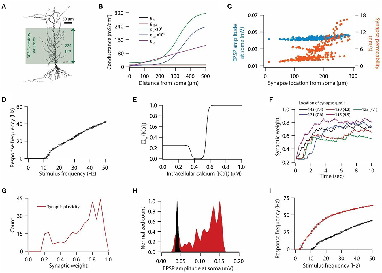
Figure 1. Synaptic plasticity disrupts input/output response homeostasis. (A) 3D reconstructed morphology of CA1 pyramidal neuron used in this study. (B) Distribution of various voltage-gated ion channels along the apical side of dendritic arbor. (C) Somatic EPSP amplitudes (cyan) of 303 synapses located across the apical dendritic arbor [green region in (A)] and their corresponding maximum permeability values (orange). (D) Input/output relationship of the model neuron under the baseline condition. All synapses were stimulated at a given frequency with stimulation timings drawn from the independent Poisson distribution. Stimulation of a synapse at a given frequency was repeated 10 times. Data is presented as mean ± SD. (E) Ω-function used in this study to update synaptic weight as a function of intracellular Ca++ concentration. (F) Example traces for evolution of synaptic weights recorded at various locations. Each of the 303 synapses was activated at a given frequency, assigned from a uniform distribution of 4–12 Hz range. The stimulation timings of each synapse were Poisson distributed. Number within parenthesis against distance denotes the stimulus frequency. (G) Distribution of final synaptic weights across all 303 synapses. Bin size 0.05. (H) Distribution of somatic EPSP amplitudes of 303 synapses under the baseline condition (black) and after synaptic plasticity (red). Bin size 5 μV. (I) Input/output response profiles of the model neuron under baseline condition (black) and after synaptic plasticity (red). Data is presented as mean ± SD.

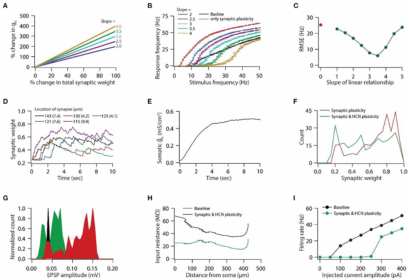
Figure 2. Synaptic plasticity accompanied with HCN conductance plasticity enables homeostasis of input/output response profiles. (A) Example graph of linear relationship between percentage change in total synaptic weight and percentage change in HCN conductance for various slopes. (B) Input/output response profiles of the model neuron under baseline condition (black), after only synaptic plasticity (red) and after synaptic and HCN conductance plasticity for various slopes of the linear relationship (A). Data is presented as mean ± SD. (C) Root mean squared error (RMSE) between baseline input/output response profile and response profile obtained after synaptic and HCN conductance plasticity (green trace) as a function of slope of the linear relationship (A). Red dot denotes RMSE between baseline input/output response profile and response profile obtained after only synaptic plasticity (Figure 1I). (D) Example traces for evolution of synaptic weights recorded at various locations (same as in Figure 1F). Number within parenthesis against distance denotes stimulus frequency in Hz. (E) Example trace of evolution of somatic HCN conductance during synaptic and HCN conductance plasticity for optimal slope (3.5) to yield RMSE minimization (C). (F) Distribution of final synaptic weights across all 303 synapses after only synaptic plasticity (red) and after synaptic and HCN conductance plasticity (green). Bin size 0.05. (G) Histogram of somatic EPSP amplitudes of 303 synapses under baseline condition (black), after synaptic plasticity (red) and after synaptic and HCN conductance plasticity (green). (H) Input resistance along the neuronal trunk computed under baseline condition (black) and after synaptic and HCN conductance plasticity (green). (I) Intrinsic firing rate profile at soma under baseline condition (black) and after synaptic and HCN conductance plasticity (green).

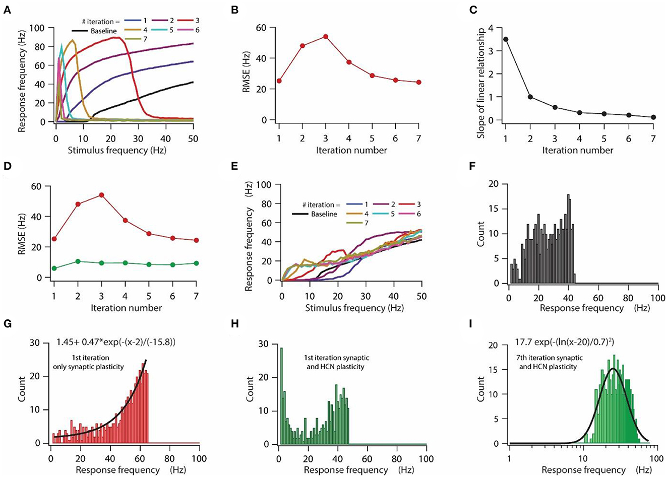
Figure 3. HCN conductance plasticity along with synaptic plasticity maintains homeostasis of input/output response profile during repeated synaptic stimulation. (A) Input/output response profiles of the model neuron under baseline condition (black) and after various iteration of synaptic stimulation. Note the complete cessation of response firing rate after 5th, 6th, and 7th iteration. Stimulation patterns for inducing synaptic plasticity of all synapses were same across all iterations. (B) RMSE between baseline input/output response profile and response profile obtained after repeated synaptic plasticity. (C) Optimal slope of the liner relationship between synaptic and HCN conductance plasticity as a function of the number of iterations of synaptic stimulation for minimizing RMSE. (D) RMSE between baseline input/output response profile and response profile obtained after synaptic and HCN conductance plasticity (green trace) as a function of the number of iterations of synaptic stimulation. Red trace same as in (B). (E) Input/output response profile of the model neuron under baseline condition (black) and after various iterations of synaptic stimulation under the condition of synaptic and HCN conductance plasticity. (F–I) Distributions of response frequencies computed across all stimulus frequencies and trials under baseline condition (F), 1st iteration of only synaptic plasticity (G), 1st iteration of synaptic and HCN conductance plasticity (H) and 7th iteration of synaptic and HCN conductance plasticity (I). Bin size 1 Hz.

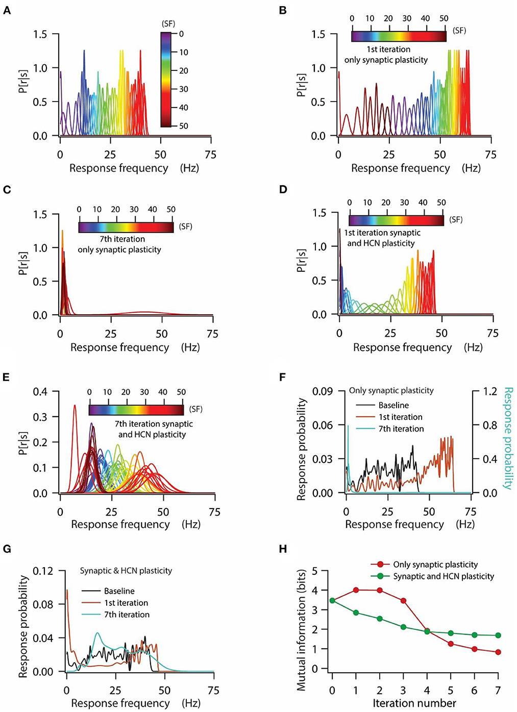
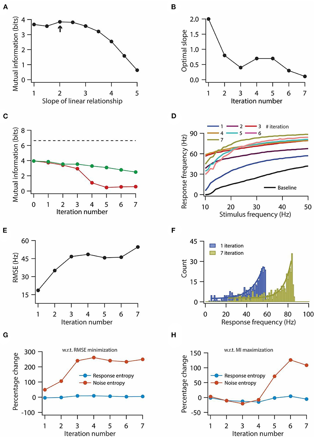
Figure 4. HCN conductance plasticity along with synaptic plasticity maintains homeostasis of input/output response profiles at the expense of mutual information transfer. (A) Distribution of probability of response firing rates for various stimulus frequencies (p[r|s]) under baseline condition. (B, C) Distribution of probability of response firing rates for various stimulus frequencies (p[r|s]) after 1st iteration (B) and 7th iteration (C) of only synaptic plasticity. (D, E) Distribution of probability of response firing rates for various stimulus frequencies (p[r|s]) after 1st iteration (D) and 7th iteration (E) of synaptic plasticity along with HCN conductance plasticity. (F) Probability distribution of various response firing rates under baseline condition (black) and after 1st iteration (brown) and 7th iteration (cyan) of only synaptic plasticity. (G) Probability distribution of various response firing rates under baseline condition (black) and after 1st iteration (brown) and 7th iteration (cyan) of synaptic plasticity along with HCN conductance plasticity. (H) Mutual information as a function of repeated iterations with introducing only synaptic plasticity (red) and repeated iterations with introducing synaptic and HCN conductance plasticity. Zero iteration denotes baseline condition.

Figure 5. Optimization of slope for information maximization also leads to a decrease in information transfer during repeated synaptic stimulation. (A) Mutual information as a function of slope of the linear relationship between synaptic and HCN conductance plasticity. Arrow indicates the optimal slope. (B) Optimal slope of the liner relationship between synaptic and HCN conductance plasticity as a function of the number of iterations of synaptic stimulation for maximizing mutual information transfer. (C) Mutual information transfer as a function of the number of iterations of synaptic stimulation under the condition of optimal slope between synaptic and HCN conductance plasticity for maximizing information transfer (B) (green trace) and only synaptic plasticity (red). Dashed line represents theoretically maximum information transfer computed under the assumption of zero noise entropy and uniform distribution of response probability within the range of 1–100 Hz of response frequencies. (D) Input/output response profiles of model neuron under baseline condition (black) and after various iterations of synaptic stimulation under the condition of optimal slope between synaptic and HCN conductance plasticity for maximizing information transfer (B). (E) RMSE between baseline input/output response profile and response profile obtained after synaptic and HCN conductance plasticity, as a function of the number of iterations of synaptic stimulation under the condition of optimal slope between synaptic and HCN conductance plasticity for maximizing information transfer (B). (F) Distributions of response frequencies computed across all stimulus frequencies and trials for 1st and 7th iteration of synaptic and HCN conductance plasticity. Bin size 1 Hz. (G, H) Percentage change in response and noise entropy as a function of the number of iterations of synaptic stimulation under the condition of RMSE minimization (G) and maximization of mutual information transfer (H).

The increase in maximal h conductance along the somato-apical axis as a function of radial distance from the soma, x, was modeled using the following formulation:

g¯h(x)=h-gB (1+h-F1+exp((h-d-x)/h-k))    (4)

where h – gB denotes maximal h conductance at the soma, set to be 25 μS/cm2, and h – F (=12) formed fold increase along the somato-apical axis. Half-maximal distance of g¯h increase, h – d was 320 μm, and the parameter quantifying the slope, h – k was 50 μm. To accommodate the experimental observations regarding changes in V1/2 of the activation of h conductance at various locations along the somato-apical trunk (Magee, 1998), the half-maximal activation voltage for h channels was −82 mV for x ≤ 100 μm, linearly varied from −82 to −90 mV for 100 μm ≤ x ≤ 300 μm, and −90 mV for x > 300 μm.

The CaT conductance gradient was modeled as a sigmoidal increase with increasing radial distance from the soma, x:

g¯CaT(x)=T-gB (1+T-F1+exp((T-d-x)/T-k))    (5)

where T – gB denotes maximal CaT conductance at the soma, set to be 80 μS/cm2, and T – F (=30) formed fold increase along the somato-apical axis. Half-maximal distance of g¯CaT increase, T – d was 350 μm, and the parameter quantifying the slope, T – k was 50 μm. These parametric constrains accounted for the experimental constraints on the coexistence of the six functional maps along the same somato-apical trunk (Rathour and Narayanan, 2014).

For simulations involving Gaussian-modulated synaptic inputs (Figures 6, 7), the parameters used for kinetics, distributions, and maximal conductances of KA, CaT, and HCN channels were the same as aforementioned, whereas maximal Na and KDR conductances were set at 15.4 and 2 mS/cm2, respectively. After changing these conductances, the model neuron was able to satisfy experimental constraints on the coexistence of the six functional maps along the same somato-apical trunk.

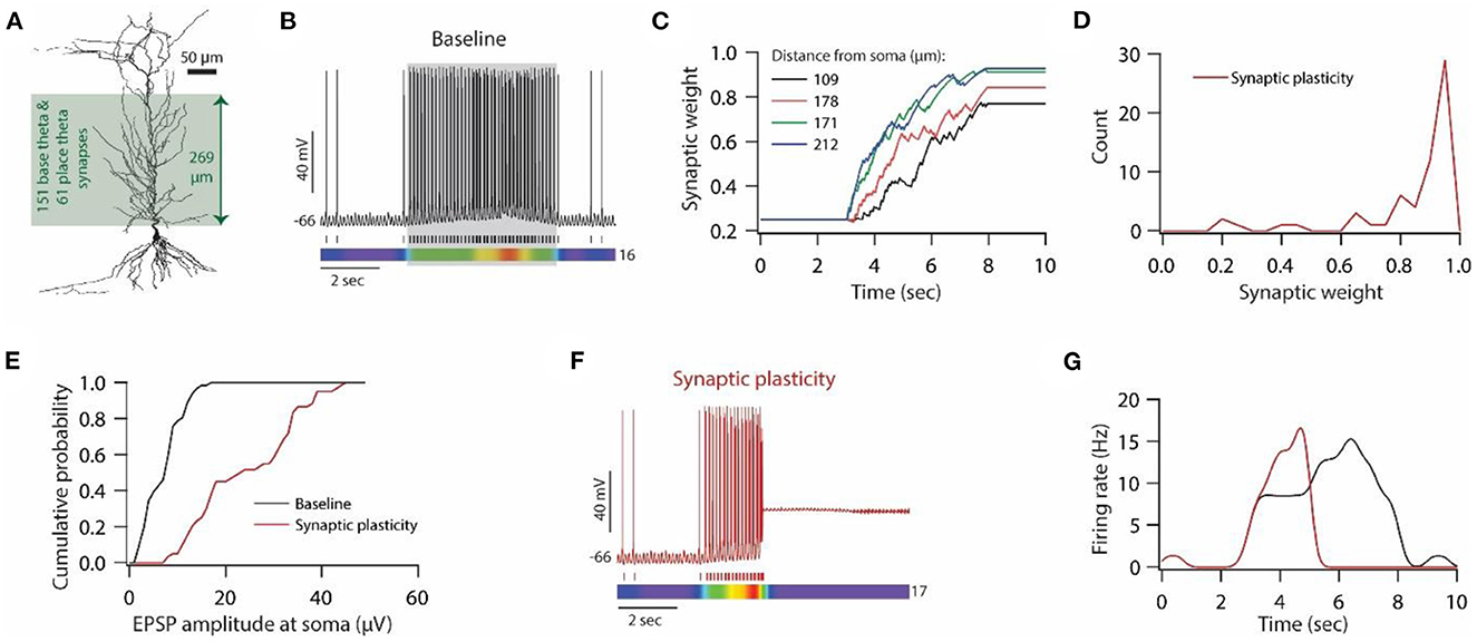
Figure 6. Synaptic plasticity disrupts place field activity in the model neuron. (A) 3D reconstructed morphology of CA1 pyramidal neuron used for simulating place field activity. (B) Top; Voltage trace recorded during Gaussian- modulated stimulation of base and place theta synapses along with asymmetric depolarizing ramp current injection at the soma under baseline condition. Middle; Spike timings. Bottom; kymograph of firing rate. Number at the right denotes the maximum firing rate in Hz. (C) Example traces for evolution of synaptic weights recorded at various locations. (D) Distribution of final synaptic weights across all place theta synapses. Bin size 0.05. (E) Cumulative probability distribution of somatic EPSP amplitudes of place theta synapses under the baseline condition (black) and after synaptic plasticity (red). Bin size 5 μV. (F) Top; Voltage trace recorded during Gaussian-modulated stimulation of base and place theta synapses along with asymmetric depolarizing ramp current injection at the soma under synaptic plasticity condition. Middle; Spike timings. Bottom; kymograph of firing rate. Number at the right denotes the maximum firing rate in Hz. (G) Place field activity under baseline condition (black trace) and after synaptic plasticity (red trace).

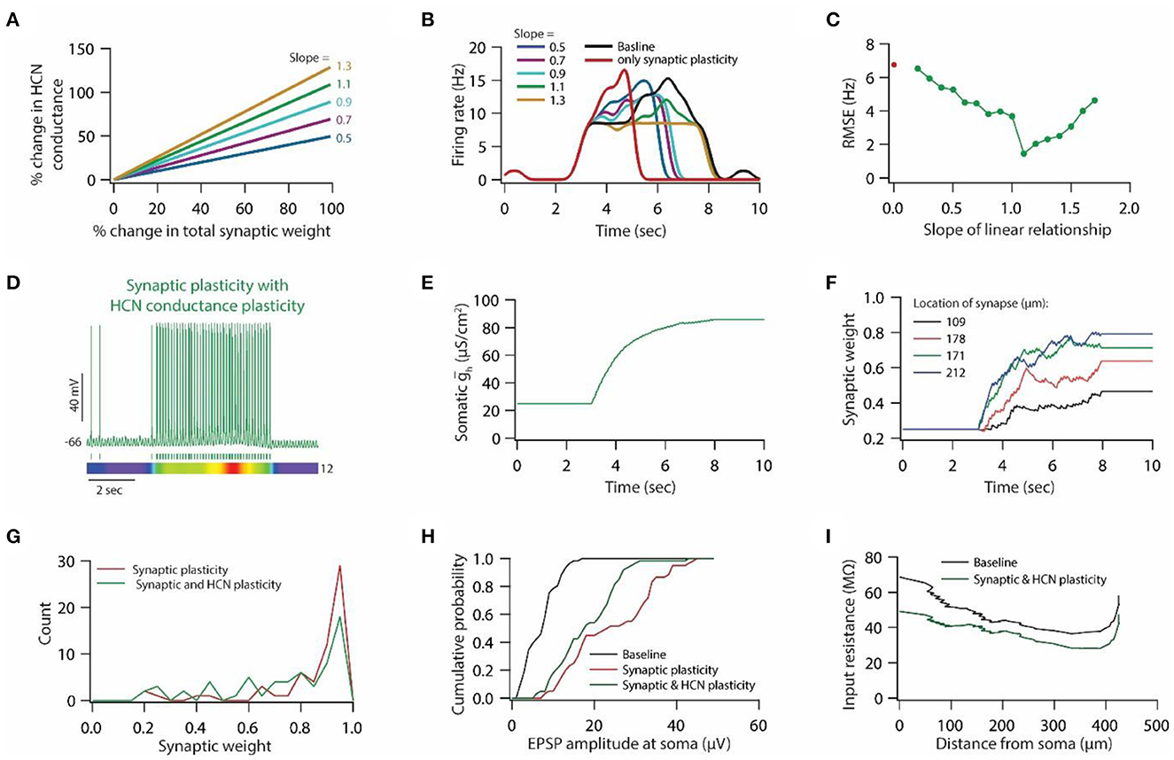
Figure 7. HCN conductance plasticity along with synaptic plasticity restores place field activity. (A) Example graph of linear relationship between percentage change in total synaptic weight and percentage change in HCN conductance for various slopes. (B) Place field profiles of model neurons under baseline condition (black), after only synaptic plasticity (red) and after synaptic and HCN conductance plasticity for various slopes of the linear relationship. (C) RMSE between baseline place field profile and place field profile obtained after synaptic and HCN conductance plasticity (green trace) as a function of slope of the liner relationship. Note, optimal slope is at 1.1. Red dot denotes RMSE between baseline place field profile and place field profile obtained after only synaptic plasticity (Figure 6G). (D) Top; Voltage trace recorded during Gaussian-modulated stimulation of base and place theta synapses along with asymmetric depolarizing ramp current injection at the soma under the conditions of synaptic and HCN conductance plasticity for slope 1.1 (optimal slope) of linear relationship. Middle; Spike timings. Bottom; kymograph of firing rate. Number at the right denotes maximum firing rate in Hz. (E) Evolution of somatic HCN conductance during synaptic and HCN conductance plasticity for slope 1.1 (optimal slope) of linear relationship. (F) Example traces for evolution of synaptic weights recorded at various locations (same as in Figure 6C). (G) Distribution of synaptic weights across all place theta synapses after synaptic plasticity (red) and after synaptic and HCN conductance plasticity (green). Bin size 0.05. (H) Cumulative probability distribution of somatic EPSP amplitudes of place theta synapses under baseline condition (black), after synaptic plasticity (red) and after synaptic and HCN conductance plasticity (green). Bin size 5 μV. (I) Input resistance along the neuronal trunk computed under baseline condition (black) and after synaptic and HCN conductance plasticity (green).

Synapse model and distribution

A synapse was modeled as a co-localization of AMPA and NMDA receptor currents as described previously (Narayanan and Johnston, 2010; Honnuraiah and Narayanan, 2013). A spike generator was used to feed inputs to the synapses at predetermined required frequencies. The default value of the ratio of NMDA:AMPA permeability was set at 1.5. Both receptor currents were modeled based on GHK formulation. The current through NMDA receptors was a combination of Na+, K+, and Ca++, and their voltage and time dependence were described by the following equations:

INMDA(v,t)=INMDANa(v,t)+INMDAK(v,t)+INMDACa(v,t)    (6)

where

INMDANa(v,t)=P¯NMDAPNas(t)MgB(v)vF2RT    (7) INMDAK(v,t)=P¯NMDAPKs(t)MgB(v)vF2RT    (8) INMDACa(v,t)=P¯NMDAPCas(t)MgB(v)4vF2RT    (9)

where F is Faraday's constant, R is the gas constant and T is the temperature in Kelvin. P¯NMDA is the maximum permeability of NMDA receptor and the default ratio of values of PCa, PNa, and PK was set to be 10.6:1:1, respectively, owing to experimental observations (Mayer and Westbrook, 1987; Canavier, 1999). The external and internal concentrations of the various ions were set as follows (in mM): [Na]o = 140, [Na]i = 18, [K]o = 5, [K]i = 140, [Ca]o = 2, [Ca]i = 100 × 10−6. This resulted in equilibrium potentials for sodium and potassium ions +55 and −90 mV, respectively. MgB(v) and s(t) denote magnesium dependence and temporal evolution of NMDA current, respectively, and were defined as follows (Jahr and Stevens, 1990a,b):

where [Mg]o denotes extracellular magnesium concentration and was set to 2 mM.

s(t)=a[exp(-tτd)-exp(-tτr)]    (11)

where a is the normalization constant to insure that 0 ≤ s(t) ≤ 1. τr and τd denote the rise and decay time constants of NMDA receptor-mediated current, respectively, and were set to be 5 and 50 ms, respectively.

The evolution of intracellular calcium, consequent to entry from NMDA receptors and T-type Ca++ channels, was modeled as described previously (Poirazi et al., 2003; Narayanan and Johnston, 2010):

d[Ca]idt=-10,000INMDACa3.6.dpt.F+[Ca]∞-[Ca]iτCa    (12)

where τCa = 30 ms is the calcium decay time constant, dpt = 0.1 μm is the depth of the shell and [Ca]∞ = 10−4 mM is the steady-state value of [Ca]i.

The current through AMPA receptors was mediated by the combination of Na+ and K+ currents and was defined as follows:

IAMPA(v,t)=IAMPANa(v,t)+IAMPAK(v,t)    (13)

where

IAMPANa(v,t)=P¯AMPAwPNas(t)vF2RT    (14) IAMPAK(v,t)=P¯AMPAwPKs(t)vF2RT    (15)

where P¯