VIsoQLR has been developed to provide users with a graphical and interactive tool for isoform identification and quantification using LRS data generated by Nanopore or PacBio technologies. It gives a single-locus at a time analysis as the data exploration focuses on the graphical display of splice site distribution across the gene. VIsoQLR automatically detects splice site coordinates that can be fine-tuned according to the user's expertise.

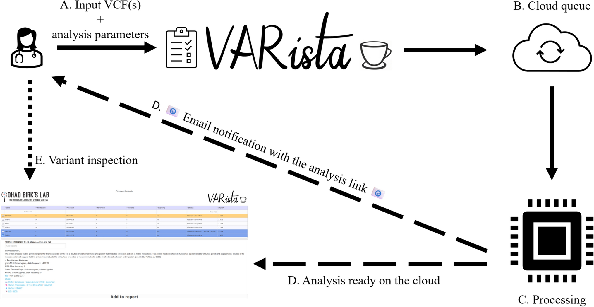
Figure 1 shows the workflow for isoform analysis using VIsoQLR. First, raw reads need to be aligned to a reference sequence. VIsoQLR has built-in options for mapping reads using GMAP (Wu and Watanabe 2005)⁠ or minimap2 (Li 2018) aligners. Next, mapped reads are uploaded, and consensus exon coordinates (CECs) are defined based on the frequency of the reads' exon coordinates (start and end positions). Start and end positions are treated independently. Some facilities for selecting final CECs are provided: (1) a frequency filter, in which start and end positions above a configurable frequency are selected as candidate CECs (by default 2%); (2) a position window, in which the user can define a window, where other non-candidate CEC (below range in the frequency filter) are merged (by default 5 nucleotides (nt) on both sides of each candidate CEC); and 3) a filter in which candidate CECs are merged into the most frequent one if they are closer than a given distance (by default 3 bases). In addition, VIsoQLR allows the user to change any parameter that defines CECs automatically and to add, delete and edit them manually. Known splice sites can also be uploaded in a file. Thus, once the consensus start and end positions are selected, the exons are defined accordingly, and reads with the same exons are considered the same isoform. The final isoform collection is defined, presented and quantified. Reads that do not fit into the delimited exons are not considered in this isoform collection, although they could be recovered if other VIsoQLR configuration is applied. Any change in exon coordinates makes isoforms redefined and quantified again on the fly.

Workflow for isoform detection and quantification using VIsoQLR. Sequenced long-reads are mapped to generate a BAM, GFF3 or BED6 file containing the coordinates of all transcripts and exons. The frequency of each exon's start and end coordinates are calculated with all reads. The selection of the consensus exon coordinates (CEC) includes the application of several optional features: (1) frequency threshold, which selects the most frequent ones; (2) window definition, where a window is defined around each candidate CECs so that close non-candidate CES are assigned to the nearest candidate CECs; (3) candidate CECs merge, where very close candidate CECs are merged into the most frequent one. Once the final CECs are defined, they are assigned to all read coordinates to define consensus exons and isoforms. Transcripts with all exons fully delimited by CECs are grouped into isoforms for quantification

VIsoQLR user interface has two working tabs, the mapping tab, where users can obtain mapped sequences from raw sequencing files using two aligners (GAMP or minimap2), and the isoforms analysis tab, which performs the VIsoQLR tasks providing its main features. In addition, external mapping can be uploaded as BAM, BED6, or GFF3 format.

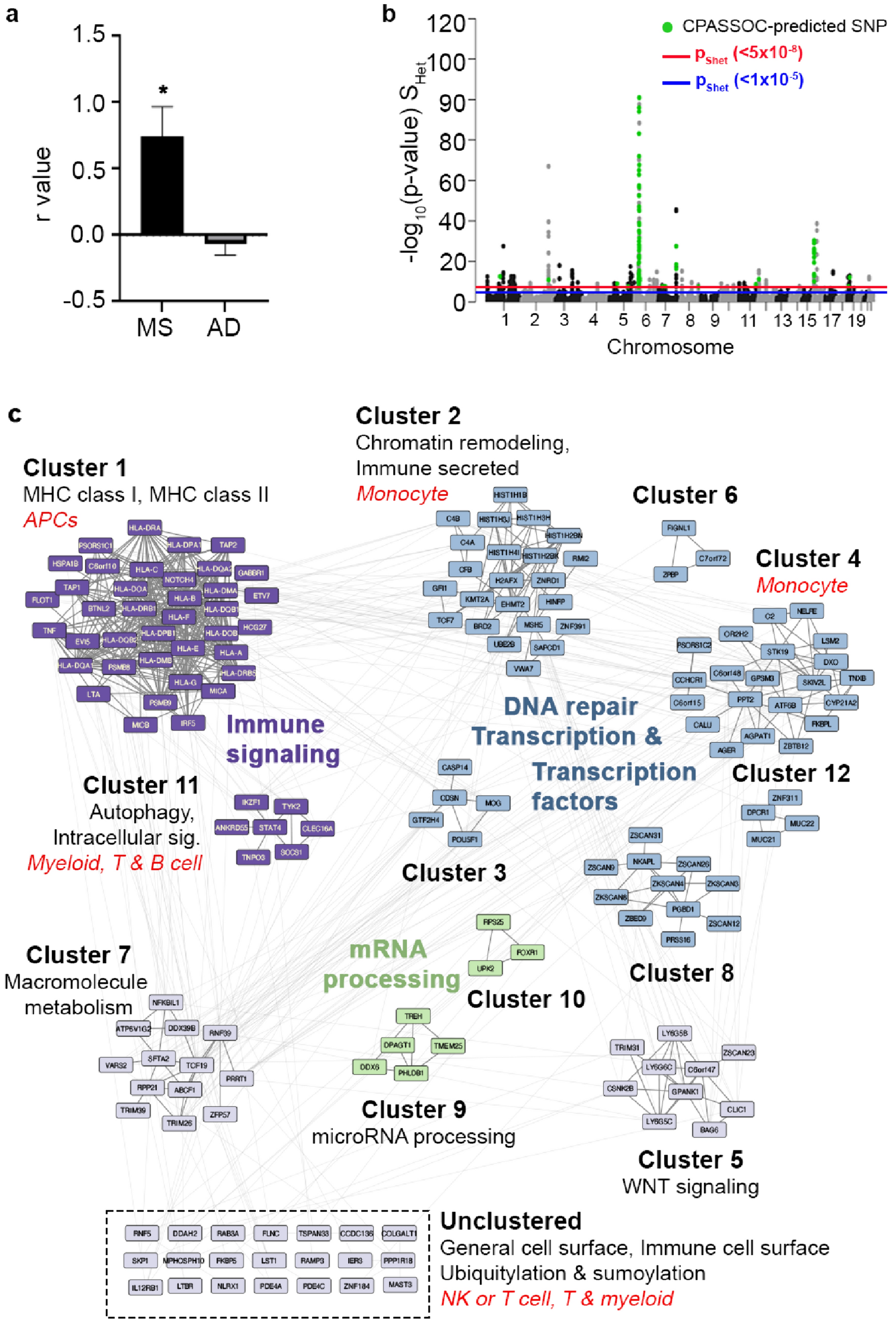
The control panel of the isoform analysis tab is shown in Fig. 2 (the complete VIsoQLR user interface of the isoform analysis tab is shown in Figure S1). To start the analysis, the user submits the aligned sequences (GFF3, BED6, or BAM formats are allowed) at the top of the control panel (Fig. 2a). Next, the different sequences submitted are displayed in a drop-down menu in the analysis bounding section (Fig. 2b). Sequences are analyzed one at a time on user request. VIsoQLR also allows to restrict analysis to specified regions, for instance to exclude exons coming from a vector or to focus on the splicing events of specific exons. Lastly, in this section, the user has the option to use only full-length PCR sequences. In the “Exon coordinates” menu (Fig. 2c), user can fine-tune the detection of splice sites. Here, options include different approaches to select CECs, such as setting up a minimum percentage of reads supporting the start and end exon coordinates, defining the size of the windows, or merging close CECs. In this control panel section, the user can upload previously defined exon coordinates (“Custom exon coordinates” menu) that replace or are merged with the automatically detected CECs performed by VIsoQLR.

Control panel of the user interface of VIsoQLR. For visualization purposes, the control panel shown in the application as a single column is here split into six subpanels. a Input subpanel where users can select the input file format and upload the aligned sequences. b Analysis bounding subpanel allows the analysis of the gene and sequence area. It also contains an option to analyze only the full-length PCR sequences. c Exon coordinates subpanel, with the option to automatically detect consensus exon coordinate (CEC). d External isoforms subpanel, where users can upload known or previously defined transcripts as a reference to curate the isoforms detected by VIsoQLR. e Display options subpanel. Here the user can filter the isoforms to be displayed based on their abundance and fine-tune the graphics. f Download prefix subpanel is used to indicate the prefix of all downloadable tables and figures

VIsoQLR also support plotting known or previously analyzed transcripts for visual comparison with the isoforms detected in the experiment under analysis. They can be submitted in GTF, or GFF3 format (“Load transcripts from file” menu) (Fig. 2d) and are displayed justified above isoforms with the same exon color codes to facilitate a direct comparison. Along with the transcript ID and size, it is possible to specify additional information about the transcript to be displayed. This information is stored in the last column of these two file formats. Visualizing a reference set of isoforms can help compare new results with previous data using VIsoQLR, those obtained with other software, or known transcripts.

The visual representation of isoforms can be adapted to the user’s requirements using the “Display option” menu (Fig. 2e). Lastly, all results, including figures and tables, can be downloaded by setting their prefix in the “Output prefix” menu (Fig. 2f).

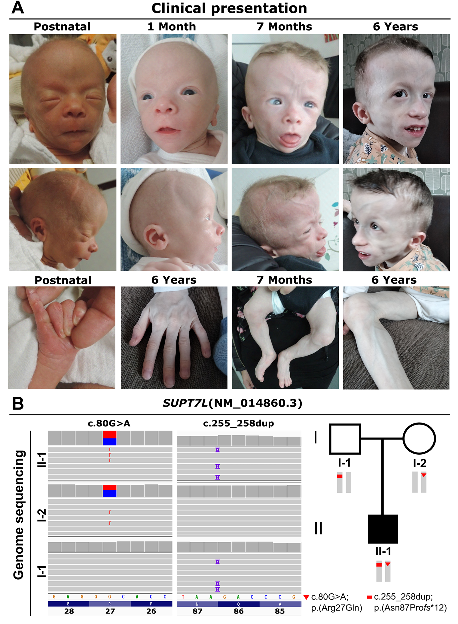
Figure 3a shows the collection of isoforms detected by VIsoQLR, including their exon configuration, coordinates, lengths and relative quantification as provided by the software. Here, isoforms detected by an external method uploaded by the user for reference or comparison purposes are shown. The exons of the uploaded isoforms are justified by those detected by VIsoQLR. Color coding is applied to represent identical exons. Below, the start (in blue) and end (in red) exon sites are shown as peaks. The height of the peaks represents the percentage of reads mapped with the same position. A zoom and graphical selection of regions is also provided for close inspection of details. Selected CECs are marked with a dot, and when hovered cursor over, these dots display a tag with the exact coordinates and the percentage of reads supporting it. The figure can be downloaded as an HTML file maintaining all the dynamic properties and a static figure in many formats in the desired size.

VIsoQLR results panel. a Display subpanel containing the isoforms detected by VIsoQLR, including their exon configuration, coordinates, lengths and relative quantification. If uploaded by the user, externally defined isoforms are displayed. The color code is used to identify identical exons. Below isoforms, the frequency of start (blue) and end (red) coordinates are shown. The consensus exon coordinates (CECs) are marked with a dot on each bar, and the exact coordinate and frequency are displayed with the cursor over. All the plots are aligned on the x-axis. This plot can be downloaded as a dynamic figure in HTML or as a static figure in multiple formats in a configurable size. b CECs are displayed in two tables (for start and end coordinates) with “Breakpoint”, “Lower limit”, and “Upper Limit” information that can be edited. The number of reads at the exact CECs and corresponding intervals are displayed. These coordinates can be downloaded as a single table. c Extra isoform and exon information regarding their lengths and abundances is displayed and can be downloaded in multiple formats

The consensus positions of the start and end exon are shown in two separate tables (Fig. 3b). Their coordinates, as well as the window defining them, can be edited directly in these tables. The manual edition of start and end positions automatically redefines the exons and isoforms and recalculates their relative abundance. These tables provide additional information on the size and abundance of isoforms and exons (Fig. 3c).

Spike-In RNA Variants (SIRVs) are a collection of synthetic transcripts with known concentrations used for quality control in RNA sequencing. To assess the detection and quantification of isoforms of our software, we analyzed public PacBio long-read sequencing data and tested the performance of three software (VIsoQLR, FLAIR and StringTie2) in detecting isoforms from the SIRV Isoform Mix E0 (Lexogen), containing 69 transcripts from seven genes (see Table S1 for mapped read sequencing metrics). FLAIR (Tang et al. 2020)⁠ and StringTie2 (Kovaka et al. 2019)⁠ are the most popular tools in whole transcriptome analysis. FLAIR requires exon coordinates to be provided as input. VIsoQLR and StringTie2 infer them from the sequence distribution. File S1, File S2 and File S3 contain the isoforms detected by VIsoQLR, FLAIR, and StringTie2, respectively.

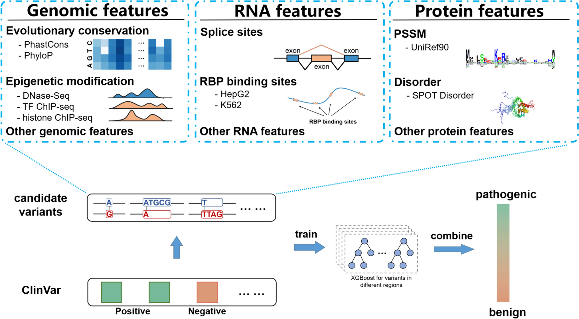
Figure 4 shows the abundance of each isoform (relative to the gene) of the detected transcripts, which intersect more than 99% of the base positions reciprocally with the gold standard (theoretical coordinates) (Table S2 contains the absolute values). Isoforms SIRV701 and SIRV705, and SIRV604 and SIRV612 were merged into two unique isoforms as they intersect in 99.92% and 99.22%, respectively, and our evaluation criteria cannot distinguish transcripts matching either of these isoforms. VIsoQLR detected 49 (72%) out of the 68 isoforms from the seven SIRVs, FLAIR detected 37 (54%), and StringTie2 12 (18%) (see Table S3 containing the total number of detected isoforms and for each SIRV). The cosine similarity of the abundances between the gold standard and VIsoQLR, FLAIR, and StringTie2 was 0.78, 0.68, and 0.42, respectively, with the partial highest similarity being 0.97 achieved with VIsoQLR in SIRV7 (Table S4). Using minimap2 as sequence mapper for all three software, the results remain similar: VIsoQLR detected 48 out of 68 isoforms (71%), FLAIR 35 (51%), and StringTie2 15 (22%), see Figure S2.

Isoform abundance in the gold standard, VIsoQLR, FLAIR, and StringTie2. The relative abundance of 68 isoforms in seven Spike-In RNA Variants (SIRVs) sequenced in a RNASeq experiment using PacBio is shown as detected by the three programs together with their theoretical concentration. All transcripts have equimolar concentrations. Transcripts were considered identical if they intersected 99%. SIRV701 and SIRV705, and SIRV604 and SIRV612 were merged as the comparison methodology used does not differentiate transcripts matching either of these isoforms, as they intersect over 99% of their bases

The relative isoform abundance for different values of the “read threshold” in VIsoQLR is represented in Figure S3. The number of isoforms detected out of the 68 SIRV transcripts was 65 (96%), 63 (93%), 59 (87%), 49 (72%), and 41 (60%), with cosines similarities being 0.81, 0.81, 0.80, 0.78, 0.74 for “read threshold” values of 0.25%, 0.5%, 1%, 2%, and 3% respectively (Table S5, Table S6 and Table S7).

With these results on hand, we now illustrate the usage of VIsoQLR in the same PacBio RNASeq experiment analyzing isoforms of two genes, PAX6 as an example of a low expressed gene, and TP53, having an average expression. For both genes we show results with a “read threshold” of 3%. In the case of PAX6 we manually merged the exon coordinates at the beginning, and at the end of the first and last exon respectively. PAX6 has a total of 45 mapped reads and the most abundant detected isoform correspond to the canonical transcript (9 reads, 45%). The rest of the isoforms are supported by 2 (10%) or 1 (5%) reads (Figure S4a). TP53 has 450 reads mapped. The most abundant detected isoform has 166 reads (88.8%) and again corresponds to the canonical transcript. The rest of the isoforms are supported with less than 4 reads (Figure S4b).

To show the applicability of VIsoQLR, we performed a multi-exonic minigene assay for exons 5 to 7 of the PAX6 gene using DNA from a healthy individual. The design of our cloned sequence in the exon trapping expression pSPL3 vector is depicted in Fig. 5a. We sequenced the amplified cDNA on a MinION flow cell and mapped the generated reads with GMAP (see Table S1 for mapped read sequencing metrics). The aligned reads were uploaded into VIsoQLR, and isoforms were calculated using default parameters and keeping only full-length PCR transcripts. To have an external reference of the methodology to detect exons and characterize isoforms, we applied StringTie2 to the same data (see Materials and methods). In Fig. 5b, we show isoforms detected by VIsoQLR at the top, justified with the results obtained by StringTie2 that were uploaded using the “Load transcripts from file” menu. Both tracks show isoforms with an abundance above 1%, and they are sorted decreasingly by this field (see Table S8 and Table S9 with the absolute abundance values for all detected isoforms). The splicing isoforms from this sample were additionally analyzed by semi-quantitative capillary electrophoresis (CE) of fluorescent amplicons to estimate the proportion of each isoform and compare it with the results obtained by VIsoQLR. The fluorescent emission peaks of each isoform are represented in the electropherogram in Fig. 5c.

Minigene design and isoforms detected from the splicing assay. a The exon trapping vector pSPL3 contains exons 5 to 7 of PAX6 (NM_000280.4). This vector contains a SV40 promoter, SD6 (splice donor 6) and SA2 (splice acceptor 2), and the Ampicillin resistance gene (Ampr). The size in base pairs (bp) of the PAX6 insert and the pSPL3 vector are shown. The forward (SD6-F) and reverse (SA2-R) primers are indicated. The amplified transcripts of the minigene are composed of SD6, E5 (exon5), E5a (alternative exon5), E6 (exon6), E6d (partial deleted exon 6), E7 (exon7), * (artifact exon), and SA2. b The isoforms detected by VIsoQLR are shown on the top track, including their exon configuration, coordinates, lengths and relative quantification. On the bottom track, isoforms detected by StringTie2 are shown. Only isoforms above 1% are represented and sorted by abundance. The color code is used to identify identical exons. c Semi-quantitative PCR electropherogram. The x-axis represents the migration time, which correlates with the size of the molecules. The y-axis represents the absorbance intensity in Relative Fluorescence Units (RFU). The size, in base pairs (bp), is shown at the top of each peak, along with the corresponding isoforms detected by VIsoQLR and StringTie2. ** Coordinates without well-defined peaks

VIsoQLR detects 40 isoforms (File S4), nine having an abundance above 1% of reads. In the case of StringTie2, it detects 58 isoforms (File S4), eight of them composed of more than 1% of the reads. The most abundant isoform detected by VIsoQLR (53.1%) corresponds to the canonical transcript. This is composed of five exons (SD6-EXON5-EXON6-EXON7-SA2), including the two specific exons of the vector and three exons of PAX6, with a size of 776 bp. StringTie2 also reports this as the most abundant isoform (60.5%), but different start and end positions make the transcript larger (816 bp). In fact, all StrinTie2 isoforms have extra bases at the begging and end compared to VIsoQLR isoforms. This canonical isoform corresponds to CE's highest peak at 772 bp (Fig. 5b).

The second most abundant isoform (17.4%) with 575 bp detected by VIsoQLR is an alternative transcript in which the EXON6 was partially skipped due to the use of an alternative exonic donor site (Grønskov et al. 1999)⁠. This transcript also corresponds to the second most abundant isoform in StringTie2 (15.0%), with a size of 615 bp and the second highest emission peak at 569 bp in CE. The third most abundant isoform called by both methods also coincides (6.3% and 6.4% in VIsoQLR and StringTie2, respectively). This is a second canonical transcript for PAX6 in which an alternative exon 5a of 42 bp (Fig. 5a) is included (SD6-EXON5-EXON5a-EXON6-EXON7-SA2), making the isoform 818 bp long in VIsoQLR and 858 bp in StringTie2. This isoform also corresponds to the electropherogram's third highest peak of 816 bp.

Both methods also called some minor isoforms below 5%. Iso6 (3.6% and 617 bp) and Iso7 (2.5% and 892 bp) detected by VIsoQLR were also called by StringTie2, as STRG.1.4 (3.3% and 657 bp) and STRG.1.5 (3.3% and 932 bp), and correspond to in the electrophoretic peaks of 612 bp and 892 bp, respectively. However, four other minor isoforms were called by VIsoQLR but not by StringTie2. Iso4 (5.0% and 645 bp) and Iso9 (1.3% and 560 bp) appear in the electropherogram at 642 bp and 552 bp peaks, respectively. But, Iso5 and Iso8 were detected neither by StringTie2 nor CE. Finally, three isoforms (STRG.1.12, STRG.1.6, and STRG.1.7) were called only by StringTie2.