1. Introduction

Major Depressive Disorder (MDD), more commonly known as clinical depression, is a severe condition with potential morbidity and mortality, affecting and threatening millions of people worldwide. MDD is typically treated with one type of antidepressant, however, 50% to 70% of patients are shown to be categorically unresponsive to medication-based treatments (Chekroud et al., 2017; Ebrahimzadeh et al., 2021a; Leichsenring et al., 2022; Turner et al., 2022). Therefore, there has been an ongoing search for other therapeutic approaches to target patients with resistant depression. One method that has gained increasing attention as a safe alternative or complementary technique to treat MDD is repetitive Transcranial Magnetic Stimulation (rTMS; Čukić, 2020). rTMS involves a series of short magnetic pulses directed to the brain to stimulate nerve cells. The magnetic pulses stimulate area neurons and change the functioning of the brain circuits involved. This method is a noninvasive treatment that directs magnetic pulses at the left or right dorsolateral prefrontal cortex (DLPFC) at regular intervals to stimulate neurons and trigger action potentials. It may be used as an adjunctive therapy to increase or hasten the efficacy of conventional pharmacotherapy through changing and modulating cortical activity. The overall effectiveness and limited side effects of rTMS have been established in several studies. Nonetheless, clinicians prescribe rTMS after conducting a thorough assessment and a series of trial-and-error tests to improve diagnostic accuracy and treatment outcomes and, importantly, to prevent patient relapse which may be the case if the patient is unresponsive to rTMS. This calls for developing indicators that can help with predicting rTMS response in order for patients to benefit from the merits of this treatment and avoid costly, ineffective procedures. Neurophysiological modalities, including fMRI and EEG, have been used to this end, between which, EEG, being more widely available and cost-effective, makes a more robust biomarker (Bachmann et al., 2013; Patel et al., 2015; Redlich et al., 2016; Wade et al., 2016; Čukić et al., 2020). This is why an increasing number of studies have applied EEG-based machine learning techniques and statistical methods to distinguish rTMS responders from non-responders (Bares et al., 2007; O’Reardon et al., 2007; Khodayari-Rostamabad et al., 2011; Arns et al., 2012, 2014; Kito et al., 2012).

The literature also includes similar efforts to determine the responsiveness of other approaches to resistant MDD treatment. A number of studies, such as Bares et al. (2007) have dealt with regarding changes in QEEG prefrontal cordance as a predictor of response to antidepressants. The effectiveness of selective serotonin reuptake inhibitors (SSRI), as another potential predictor of treatment response, has been investigated in the study of Khodayari-Rostamabad et al. (2013), where Khodayari-Rostamabad et al. obtained the patient’s initial EEG and used it to extract features and perform a mixture of factor analysis (MFA) model. This led to a classification accuracy of 87.9%. SSRI efficacy was also examined in another study, where logistic regression (LR) was applied to wavelet features of baseline EEG, producing an accuracy of 87.5% (Mumtaz et al., 2017). Transcranial Direct-Current Stimulation (tDCS) is another treatment for mood and cognition improvement in patients with MDD, which was the focus of Al-Kaysi et al. (2017). The authors made use of Linear Support Vector Machine (LSVM), Linear Discriminant Analysis (LDA), and neural networks to classify features extracted from EEG and achieved an accuracy of 76% and 92% in mood and cognition labeling, respectively.

As for rTMS, the authors (Cao et al., 2018a) provided a meta-analysis reporting relatively low rates of 40.9% and 16.4% for response and remission, respectively. Bailey et al. (2018) examined EEG recordings when participants were completing a Working Memory (WM) task and predicted rTMS response with an accuracy of 91%. In another effort, they obtained resting state EEG at baseline and 1 week after the start of the treatment and combined mood and EEG features using an LSVM classifier. This yielded a classification accuracy of 86.6% (Bailey et al., 2019). The extracted EEG features they used included EEG power and weighted phase lag index (wPLI) in alpha and theta (Bailey et al., 2019) and gamma (Bailey et al., 2018) frequency bands, alpha peak frequency (iAPF), and frontal theta cordance (Bailey et al., 2019; Jaworska et al., 2019). The literature also includes other EEG features used for the same purpose such as power spectral features (Khodayari-Rostamabad et al., 2013; Al-Kaysi et al., 2017), coherence (Khodayari-Rostamabad et al., 2013; Mumtaz et al., 2017), mutual information (MI; Khodayari-Rostamabad et al., 2013), nonlinear features (Hasanzadeh et al., 2019), time-frequency processing (Ebrahimzadeh et al., 2021a), and wavelet coefficients (Mumtaz et al., 2017). Among these, EEG power in different frequency bands and their combinations have received a lot of attention in predicting MDD treatment (Suffin and Emory, 1995; Knott et al., 2000; Cook et al., 2002; Bruder et al., 2008; Spronk et al., 2011; Tenke et al., 2011; Arns et al., 2012; Pellicciari et al., 2013; Wade et al., 2016; Lebiecka et al., 2018). For instance, treatment response was shown to be associated with cordance measures (Leuchter et al., 1994) and, in another study, with an Antidepressant Treatment Response (ATR) index (Iosifescu et al., 2009). Olejarczyk et al. (2020) evaluated the impact of rTMS on functional connectivity in MDD and bipolar disorder by directed transfer function and indices based on graph theory.

A number of studies have brought their attention to the non-Gaussian, higher-order nature of EEG to discover supplementary information that is not detected in the power spectrum. Adopting this view, Hasanzadeh et al. (2019) used non-linear and bispectral features to classify rTMS response.

Furthermore, a large strand of literature employs three prefrontal electrodes, i.e., FP1, FP2, and FPz, to extract predictive features, as the frontal lobe is believed to contain significant changes in MDD. Such studies tend to limit their analyses to the outcome of those electrodes, which could be interpreted as a simplification of the matter: there is little guarantee that the frontal components would not affect the channels from other areas namely the central, parietal, temporal, and occipital. It can then be stated that the components from the frontal lobe are more involved than those from other areas. Identifying these components and extracting features from their time series could lead to more realistic results compared to those of the other EEG channels. In other words, the frontal components form a neural network, which is involved in the rTMS treatment, and the EEG channels reflect their activity. That said, this article tries to shift the focus to the component domain. To do this, we first had the channels decomposed to their components and identified the appropriate components through analyzing their locations and the dipoles related to the MNI model. We then used the time series of the selected components to extract features and performed the classification. To choose predictive features for rTMS treatment response, we investigated a relatively comprehensive set of component’s time-series features including spectral, bispectral, and nonlinear features, namely bispectrum features, Lempel-Ziv Complexity (LZC), correlation dimension (CD), fractal dimension (FD), component power in all frequency bands (delta, theta, alpha, and beta), and frontal and prefrontal cordance in the theta band, all extracted from pretreatment resting EEG. In addition to classification, we performed a statistical test to evaluate the differences of features in two groups of responders (R) and non-responders (NR). Ultimately, we employed a Genetic Algorithm (GA) for feature selection. To the extent of our knowledge, this is the first time that the capability of selected bispectral, nonlinear, and spectral features on the components time-series have been investigated simultaneously with the aim of treatment response prediction.

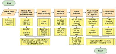
As illustrated in Figure 1, we first provide the information of participants, and the procedure of EEG acquisition. After extracting the relative components and features, we perform the classification and statistical test. Based on our classification study, we will evaluate the prediction ability of feature sets in the Results Section. The features will then be used to categorize the subjects into two groups of R and NR based on our statistical analysis. The results are elaborated in the Discussion Section where the limitations of the current study and suggestions for future work are also presented. The article is concluded in the Conclusion section.

Figure 1. Block diagram of the proposed approach for prediction of rTMS treatment response in MDD.

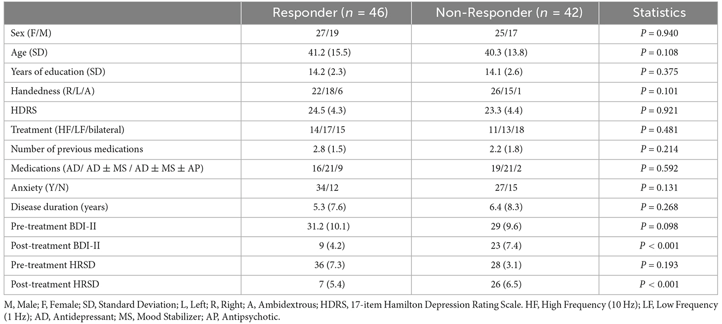
2. Methods and material 2.1. Participants

We recruited 88 patients with MDD in the age range of 18–54 years. The patients were referred to the Neuraly Clinical Neuroscience Centre, Tehran, Iran. A psychiatrist diagnosed them with MDD using the Diagnostic and Statistical Manual-IV (DSM-IV) diagnostic criteria (Segal, 2010). The Hamilton Rating Scale for Depression (HRSD) and the Beck Depression Inventory were also used to assess the participants (BDI-II). All participants have an HRSD score ≥12 and a BDI-II score ≥15. The demographic and clinical data of the participants are described in Table 1. Wilcoxon rank-sum and Friedman tests were used to compare the R and NR groups, with the results displayed in column 4 of Table 1.

Table 1. Clinical and demographic information.

In terms of age, gender, rTMS treatment features, pretreatment BDI-II and HRSD score, medications, duration of illness, length of current depression episode, and the number of previous drugs, there were no significant differences (p > 0.05) between R and NR. Only the posttreatment BDI-II and 17-item HRSD scores differed significantly (p < 0.05), with responders scoring significantly lower. The outcome of rTMS cannot be attributed to differences in depression severity of the two groups because the pretreatment BDI-II and HRSD of R and NR are not significantly different. The existence of Axis I or II disorders, substance misuse, suicide risk, unstable medical conditions, implanting devices, cardiac arrhythmia, and pregnancy are all exclusion criteria in this study. Participants having a current or previous head injury, seizures, epilepsy, or neurological diseases were also excluded from the study. In this study, 59 individuals had been on antidepressants, mood stabilizers, and antipsychotics for more than 4 weeks prior to the treatment. The Bioethics Committee of the Iran University of Medical Science authorized all experimental techniques, which followed the principles of the Declaration of Helsinki standards. All participants volunteered and provided written consent after being told about the study procedures and goals. Table 1 summarizes the demographic and clinical information of the participants.

2.2. Procedure and clinical assessment

A baseline interview was conducted with MDD patients to collect demographic and depression severity data. The 17-item Hamilton Rating Scale for Depression (HRSD; Sharp, 2015), the Montgomery-Asberg Depression Rating Scale (MADRS; Leentjens et al., 2000), and the Beck Depression Inventory-II (BDI-II; Dozois et al., 1998) were used to determine the severity of depression.

MDD patients received daily (5 days per week) unilateral left 10 Hz rTMS therapy for 3 weeks. Individuals who responded after 3 weeks were given an extra 2 weeks of titrated rTMS treatment (three sessions in week 4, two sessions in week 5), followed by another EEG session. Nonresponders were randomly assigned to continue with unilateral left 10 Hz rTMS therapy, unilateral right 1 Hz rTMS treatment, or sequential bilateral rTMS treatment consisting of right 1 Hz rTMS followed by left 10 Hz rTMS treatment for the next 3 weeks. Individuals who did not respond by week 3 but did by week 6 were given another 2 weeks of titrated rTMS treatment (three sessions in week 7, two sessions in week 8). The procedure for rTMS treatment is shown in Figure 2. The stimulation intensity was set at 110% of the resting motor threshold. The left-sided treatment consisted of 40 5-s trains separated by a 25-s break. One train of 1,200 pulses was used for right-sided rTMS. These procedures were combined in bilateral rTMS, but with only 900 right-sided pulses. The coil was held tangentially to the head and its handle facing back and away from the midline at 45°, and the rTMS was applied to the left/right DLPFC and bilateral DLPFC at a point 5 cm anterior in a parasagittal line to the motor threshold location (the left abductor pollicis brevis muscle). A TAMAS (REMED, Daejeon, South Korea) with a figure-of-eight-shaped coil (field strength 3 Tesla) delivered the rTMS. At the end of week 1 and week 3, the MADRS and BDI-II tests were redone. Individuals who had not responded by week 3 but had responded by week 6 were assessed using the MADRS, BDI-II, and HRSD at weeks 6 and 8. Anxiolytics and hypnotics were allowed at stable levels before the start of the rTMS therapy, but not 8 h before an EEG recording. During the study period and for at least 5 days before EEG recording and the first rTMS session, no antidepressants, antipsychotics, or anticonvulsants were allowed. It is necessary to mention since it can be quite a serious ethical and medical issue to prohibit the use of antidepressants for patients with depression, whose pre-treatment HRSD scores indicate severity of about 30 points, individuals who had these conditions were excluded from participating in this study. At the beginning and end of the treatment, resting EEG was obtained. The participants’ EEGs were recorded for 5 min in each session while they sat in a comfortable chair in a shielded room with their eyes closed (Ahmadlou et al., 2012; Hasanzadeh et al., 2019). The participants were told not to fall asleep during the experiment. Responding to treatment is defined as more than 50% decrease in BDI_II scores or HRSD or by BDI ≤ 8 (HRSD ≤ 7) which indicates remission (Hasanzadeh et al., 2019).

Figure 2. The procedure for rTMS treatment and the selection of two responsive (R) and nonresponsive (NR) groups.

2.3. EEG recording and pre-processing

All EEG recordings took place at the Neuraly Clinical Neuroscience Centre, Tehran, Iran. A 32-channel eWave32 amplifier was used for EEG signal recording which followed the International 10–20 System of electrode placement on the scalp. The amplifier, made by ScienceBeam, has a sampling rate of 1k samples/second, allowing us to precisely study the temporal dynamics of information processing in the brain (with a referential montage, where the reference electrode was placed in the FCz position; Raeisi et al., 2020; Seraji et al., 2021; Seraji, 2021). We applied standard pre-processing procedures in EEGLAB (available at https://sccn.ucsd.edu/eeglab/ version 2021) to reduce noise and artifacts from the EEG signals (Ebrahimzadeh et al., 2021b). First, the sampling rate of the signal was reduced to 250 Hz, and filtered by a Butterworth band-pass filter at 1–60 Hz. Then, all the channels were reviewed, and those with a standard deviation greater than ±3.1 from the mean standard deviation (across all channels) were excluded as the channels that contain artifact. For eliminating the power-line noise at 50 Hz, the Clean Line algorithm was used (Ebrahimzadeh et al., 2019a,b). The advantage of this algorithm over the notch filter is that it adaptively estimates and removes sinusoidal artifacts without creating band-holes in the EEG power spectrum (Ebrahimzadeh et al., 2021b). Next, the ICA algorithm was applied on the EEG signal and the irrelevant components corresponding to eye blink, eye movement, cardiac pulsatile, muscular tension, swallowing, or machine vibration were visually identified using the component’s scalp map, spectral power activity, and spectral power distribution (Ebrahimzadeh et al., 2019c, 2021c; Sadjadi et al., 2021). After identifying all the artifact components, the data were re-composed without them. Finally, the average reference was used to re-reference all of the data. We kept 300 s of each subject’s EEG signal to equalize the length of data for all participants, taking into account the parts of the EEG data that were eliminated.

2.4. LORETA

To determine brain electrical sources, researchers use the LORETA method (low resolution electromagnetic tomography). LORETA is a Laplacian-weighted minimum norm algorithm that relies on the patient’s prior neuroanatomical and physiological knowledge as well as a mathematical restriction. The method is based on projecting the brain’s electric activity onto all of the points in a 3D grid. Unlike dipole source modeling approaches, every site whose activity is reformed is considered a potential source (Jaworska et al., 2019). As a result, the model does not require a predetermined number of sources. The smoothest spatial distribution is chosen by minimizing the Laplacian of weighted current sources. The idea is that neighboring voxels should have an electrical activity that is as comparable as possible, such as the same orientation and activation. The LORETA approach, being time dependent, allows for an inverse solution by using spatial coefficients as input. It is sufficient to have a one-time sample to generate a combination of sources. That said, we separated EEG activities into time windows for a solution, and investigated the 5-s segments.

2.5. Independent component analysis (ICA)

Independent Component Analysis (ICA) is used for a statistical decomposition of multi-channel EEG signals for source separation. The EEG signal is made up of a variety of contributions, and utilizing this method, independent components can be isolated from the mixed signals. ICA converts a multivariate random signal into a signal with mutually independent components. We extracted the time series of each component of the DLPFC area and then elicited the features. We chose the first three components to study since each participant had at least three components in the DLPFC region, and the first three components are more likely to play a substantial role (Figure 3; Ebrahimzadeh et al., 2019a,c, 2021b,c).

Figure 3. Application of ICA on EEG after rTMS treatment. (A) Extracted components from ICA in the frontal region. (B) Extracted dipole from ICA in the frontal region. (C) Extracted components time-series from ICA in the mentioned region.

2.5.1. Region of interest (ROI)

Referring to the existing literature, we have defined a region-of-interest method to obtain the volumetric measurements of DLPFC. In a number of studies, it is shown that the DLPFC site is optimally identified as the midpoint of a line drawn between the F3 and AF3 EEG points (Fitzgerald et al., 2009; Ahdab et al., 2010; Peleman et al., 2010). In addition, authors of Paxinos and Mai (2015), Brodmann (1909), Fischl and Dale (2000), and von Economo et al. (2008) have highlighted the fact that the human cerebral cortex is a highly folded sheet of neurons with a thickness varying from 1–4.5 mm (overall average being around 2.5 mm). Considering both views, we have determined the ROI as a cylinder that has a circle centered in the middle of F3 and AF3 with a radius of 25 mm and a thickness of 2.5 mm.

2.6. Feature extraction

After extracting the time series of linked components, features extraction is the next stage in predicting treatment response to rTMS. We evaluated a total of 23 features in four categories: nonlinear, spectral, bispectral, and cordance. Each feature (excluding cordance) was computed for all selected components of both groups of R and NR. Thus, for each measure, we have a feature set containing 23 feature vectors corresponding to three components making a total of 69 features. The next sections describe the measures that were investigated.

2.6.1. Power spectrum

The signal’s power in its frequency components is represented by the power spectrum. Delta (1–4 Hz), Theta (4–8 Hz), Alpha (8–12 Hz), and Beta (12–24 Hz) are common frequency bands. The components time series were used to calculate the average powers. The power spectrum of the components bands was calculated using a Fast Fourier Transform based on the Welch method for each band of each component. The Welch’s approach separates the signal of N samples into K data segments of M samples, with D samples possibly overlapping. After that, the overlapping portions are windowed, i.e., multiplied by a symmetric bell-shaped window. The periodogram of each windowed data segment can then be computed using the discrete Fourier transform (DFT). The average adjusted periodogram of all segments is then calculated as the final estimate of the spectrum. In this study, a non-overlapped window with 1,000 samples (1 s length) was chosen for each band of each component.

2.6.2. Cordance

Cordance is a quantitative EEG approach that embodies information from the EEG spectra’s absolute and relative powers. Many researchers have used cordance as a way of distinguishing depression and predicting treatment outcomes (Bares et al., 2015; Baskaran, 2016; Bailey et al., 2018, 2019). Age, gender, and the degree of baseline depression have little impact on cordance. The ratio of the delta, theta, alpha, or beta band power over the total power in the full frequency range, which eliminates individual differences, has been termed as the relative EEG power. Some of the previous studies have shown decreased prefrontal cordance of the theta frequency band after the treatment (Cook et al., 2002; Bares et al., 2007, 2015; Cao et al., 2018b; Bailey et al., 2019). Therefore, in MDD, prefrontal theta cordance can be a documented neurophysiological biomarker for predicting response to antidepressants. In this work, theta cordance from extracted component time series in prefrontal was calculated according to the following three steps:

First, the power spectra (P) were averaged for each component. The absolute and the relative power (Ps,f and P¯s,f respectively) were expressed as:

where s is the electrode site and f and f’ are the specific frequency band and all bands, respectively.

Second, the absolute and relative EEG powers were normalized by dividing them by the maximum absolute and relative powers in each frequency band (f) as:

PRNORM(s,f)=P¯s,fmaxP¯s(3)

Finally, the cordance values at each electrode site (s) for each frequency band (f), Cs,f, were calculated as:

Cs,f=(PANORM(s,f)−0.5)+(PRNORM(s,f)−0.5)(4)

In this study, we calculated theta cordance from extracted component time series in prefrontal.

2.6.3. Nonlinear features

Various methods have been proposed over the last two decades for obtaining EEG nonlinear properties to characterize brain activities. The first and most important characteristic of EEG is its dynamic “complexity,” which may be quantified via complexity analysis. The degree of unpredictability in time series is mostly represented by the complexity analysis. In this study, we computed four nonlinear features. All nonlinear measures were calculated for epochs of component time series with the length of 3,000 samples and then have been averaged over all epochs. Thus, for every component, we have four values that are corresponding to each nonlinear measure for every subject.

2.6.3.1. Permutation entropy (PE)

Permutation entropy (PE) is a new feature extraction method, which has low computational complexity, robustness, and simplicity (Grova et al., 2008; Berger et al., 2017; Ebrahimzadeh et al., 2018a; Hasanzadeh et al., 2019; Čukić et al., 2020). It can be used to investigate the local order structure of a dynamic time series and measure the degree of regularity in the EEG data. PE turns an EEG time series into an ordinal pattern sequence. It converts non-stationary time series into a set of ordinal patterns, each of which describes the order relationship between the present and a set of equidistant previous values at a given point in time.

The PE values reported in this work were divided by log(m!) for normalization. They are dimensionless quantities in the interval [0, 1] (Berger et al., 2017).

For a scalar time series X(n) = [x (1), x (2),‥., x (n)], the reconstruction time series is:

X(i) = [x(i), x(i+τ), ..., x(i+(m+1)τ)] I = 1, 2, ... , n (m−1)τ(5)

where m is “the length of the pattern”, that is the number of sample points included in each pattern and the “time lag” (τ) is the number of samples that spanned each section of the pattern. Then, x(i) is rearranged in increasing order:

xi+j1−1τ≤xi+j2−1τ≤...≤xi+jm−1τ(6)

For m different numbers, there will be j = m! permutations. The vectors X(i) can be mapped to one of the m! permutations. Next, for the time series X(n), the probability of each permutation occurring (p) can be defined as:

where nj is the number of times the jth permutation is occurring.

The permutation entropy of the time series x(i) = [x (1), x (2), ‥., x (n)] is defined by:

Hx(m)=∑j=1m!pjln pj(8)

When the time series is random, Hx(m) approaches its maximum value of ln(m!); when the time series is regular (non-random), Hx(m) approaches zero. Finally, the corresponding normalized permutation entropy is:

The smallest value of PE is zero, which means the time series is very regular; and the largest value of PE is one, which means the time series is completely random.

2.6.3.2. Fractal dimension (FD)

Earlier research has shown that EEG complexity analysis using FD may be employed successfully in a variety of clinical settings, implying that FD could be a good indicator of the efficacy of rTMS therapy (Lebiecka et al., 2018). The level of self-similarity of a time series is measured using an FD algorithm, which relates to how many times a pattern in the time series is repeated. FD was calculated using the Higuchi’s fractal dimension (HFD) technique (Ahmadlou et al., 2012; Bachmann et al., 2013; Čukić, 2020). The signal is represented by a sequence x = [x (1), x (2),‥., x(n)], where n is the total number of samples and x(i) indicates the ith sample of x. From a given sequence, k subsequences Xmk will be defined as:

Xmk:Xm,xm+k,...,Xm+jk,m=1,2,...,k,(10)

where m is the initial time and k is the interval time.

The average length of each subsequence Xmk can be calculated according to:

Lmk=1k∑i,jkXm+ik−Xm+i−1kN−1j(12)

where N−1j is a normalization factor. The total average length for scale k, L(k), is computed as the average of the k values, for m = 1, 2, ‥., k, that is:

The calculation is repeated for k values ranging from 1 to kmax. kmax is considered to be the number when the slope of the best line fitted to the diagram of L(k) vs. 1k plotted in a log-log plane remains constant (kmax ≥2). The slope of this line is HFD of the time series L. The line is defined by the linear regression coefficient which is determined by the least squares method. kmax = 16 is shown to perform the best for this type of signal (Spasic et al., 2005; Lebiecka et al., 2018; Čukić et al., 2020).

2.6.3.3. Lempel-Ziv Complexity (LZC)

The rate at which new patterns arise in time series is indicated by a nonlinear dynamic measure. The activities of adding or removing the patterns of the underlying system are examined when employing LZC (Aboy et al., 2006). The LZC method is based on coarse-graining, which converts the signal s(n) into a limited sequence of a few symbols (Li et al., 2008). Traditionally, the coarse-graining procedure turned the signal s(i) into a binary sequence x(i) = x (1), x (2),..., x(i). By comparing the signal values with a threshold, the original signal is converted into a binary (0, 1) sequence, with the median of the signal values chosen as the threshold.

xi=Limn→∞cn=bn=nlog2n(16)

The complexity measure c(n) is normalized to b(n), to make the measurement independent of the length of the data, and LZC will be obtained by:

By transforming the signal into a finite sequence , c(n) will be the complexity of the sequence and will denote the number of distinct patterns in the sequence.

2.6.3.4. Correlation dimension (CD)

Based on embedding theory and phase space reconstruction, the correlation dimension of a dynamic system is established. Considering the state points, x(1), x(2),‥.,x(n), new m dimensional vectors can be reconstructed by choosing a time delay t and embedding dimension m.

Xi=xi,xi+t,...,xi+m−1t,     i=1,2,...,n−m−1t(18)

The correlation dimension is obtained by:

Cr,n=2nn−1∑i=1n∑j=i+1nθr−xi−xj(19) Dr, n=limr→0ln Cr, nln r(20)

where θ is the Heaviside step function which is defined as θ(x) = 0 for x < 0 and θ(x) = 1 for x > 0; C(r, n) is the correlation integral and D(r, n) is the correlation dimension. The procedure is repeated for increasing m.

2.6.4. Bispectrum features

The spectral band power can show phase variations, but does not reveal interactions between the signal’s frequency components. Note that a signal’s “shape” is determined by its phase, and signals with different wave forms might have the same power spectrum (Acharya et al., 2015).

Bispectrum is a higher-order statistical signal processing technique that examines both the amplitude and the degree of phase coupling of a signal. In the context of EEG signal categorization, bispectrum has demonstrated promising results. The two-dimensional Fourier transform of a signal’s third order correlation is defined as the signal’s bispectrum Bis(f1, f2). Bispectrum divides a signal’s skewness (third order moment) throughout all frequencies, characterizing the intensity of interaction between all frequency pairings in the target band.

Bisf1,f2=limT→∞1TEXf1+f2X*f1X∗f2(21)

where X(f) is the Fourier transform of a time series x(t), * is the complex conjugate, T represents time, and E denotes the expected value. Indeed, bispectrum indicates cross-correlation between frequency components in a two-dimensional frequency plot. The phase coupling information between the frequency components at f1, f2, and f1 + f2, can be extracted from Bis (f1, f2). The degree of phase coupling between frequencies components is obtained by the following normalized bispectrum:

Bisnormf1,f2=Bisf1,f2Pf1Pf2Pf1+f2(22)

The power spectrum is denoted by P(f), and the magnitude of the normalized bispectrum has a value between 0 and 1. The squared magnitude of the normalized bispectrum will be 1 if the Fourier components at the frequencies f1, f2, and f1+f2 are perfectly phase-coupled in every realization, and 0 if they are completely random.

To distinguish the distribution of the bispectral plots of distinct EEG data, quantitative characteristics must be defined. The bispectrum of a genuine signal is uniquely described in the triangle 0≤f2≤f1≤(f1+f2)≤1, assuming no bispectral aliasing. For characterization of the entire bispectrum, features are defined by integrating along straight lines going across the non-redundant region. Three features were collected from the bispectrum region in this investigation. These features are defined as follows.

Average of magnitude:

where L is the total number of sample points in the bispectral density array and Ω is the triangle region shown in Figure 4.

Bispectral entropies:

pn=Bisf1,f2∑ΩBisf1,f2(25) qi=Bisf1,f22∑ΩBisf1,f22(27)

where P1 and P2 are the normalized bispectral entropy and normalized bispectral squared entropy which are also between 0 and 1.

Figure 4. The non-redundant region of bispectrum plot.

2.7. Feature selection

Before performing classification, we use feature selection for two main reasons: first, to eliminate the irrelevant features which can raise the complexity of classification and lower its accuracy, and second, to address the dimensionality problem. That said, after extracting EEG features, we applied a genetic algorithm (GA) to pick out the most discriminating features. GA is a group of computational models based on natural selection and genetics laws. In a high-dimensional space, it is considered as a stochastic strategy that outperforms deterministic optimization strategies. The GA begins with a population of individuals that represent a potential solution to a particular optimization issue and evolves over generations to a group of more optimal or fit individuals. Then, it replicates the offspring using basic genetic procedures such as selection, crossover, and mutation. A fitness value is assigned to each individual or community, and the fitness of the candidate individual is assessed. Finally, GA selects the best individuals from the existing population (Amoozegar et al., 2019).

2.8. Classification

We suggested a novel strategy to predict the rTMS treatment response based on classification analysis to separate responders from non-responders by the K-Nearest Neighbor (KNN), Support Vector Machine (SVM), and Multilayer Perceptron (MLP) classifiers. We ran our analysis on a different set of extracted features from the component time series. First, we assessed the capacity of the researched features to predict treatment response by applying classification to each measure individually. Then, in a second classification study, a mixture of features from each of the four categories (nonlinear, spectral, bispectral, and cordance) were utilized to classify R and NR. Finally, we assessed a combination of all features for classifying R and NR. For all analyses, the classification process detailed below was comparable. After feature extraction, the feature sets were separately standardized by the z-score normalization to minimize amplitude variations caused to differences in subjects and electrode placements. Afterwards, we employed GA to pick the most informative features.

In all analyses, the number of features was determined by a trial-and-error method to discover a value that maximizes accuracy while avoiding overfitting of the classifier. The square root of the total number of features in the related study was used to match this ideal number of features in our analysis, except for prefrontal cordance analysis, where due to the small number of features, we used all features.

A 10-fold cross-validation method was used to assess the classifiers’ performance. Except for two or three groups, the EEG data of 88 subjects were separated into 10 parts, with the number of signals in each part being equal. The classifier was trained using nine parts and the remaining part was used to test it. This process was performed 10 times, and the average and standard deviation of accuracy, sensitivity, and specificity were obtained.

2.8.1. Multilayer perceptron (MLP)

A three-layer MLP with the error back propagation method and variable learning rate was used. For component time series (Ebrahimzadeh et al., 2011, 2018a,b, 2019d; Ebrahimzadeh and Pooyan, 2013; Nikravan et al., 2016), the input layer has the same number of nodes as the input vector length. The output layer, on the other hand, only has one node, which means that only two classes can be classified. The optimal number of neurons in the hidden layer was found by selecting and training all feasible combinations of the selected numbers of neurons in the hidden layer. It is worth noting that the entire training procedure was based only on the training data. We moved on to testing the network using the testing data after the training is completed. The network did not use the testing data while determining the best architecture to maximize the network’s generalization.

A linear transfer function and a sigmoid function were used in the output nodes and the hidden layer, respectively (Ebrahimzadeh et al., 2013). The network training continues until the error becomes less than 0.01, or 1,000 training iterations are completed (Ebrahimzadeh et al., 2014).

2.8.2. K-Nearest neighbor (KNN)