A CNN-LSTM model for six human ankle movements classification on different loads

Not only does the architecture of the neural network affect its performance, but the selection of hyperparameters is also important (Joshi et al., 2013). For the network architecture proposed in this article, the hyperparameters that needed to be considered included the following: (a) the number of layers of the network, (b) filters size, (c) kernel size, (d) pooling size, (e) stride rate, and (f) time step. At the same time, the training parameters that we needed to adjust included the following: (a) number of epochs, (b) learning rate, (c) activation function, (d) loss function, (e) batch size, and (f) dropout. The hyperparameters of our model were mainly determined with reference to previous studies and then manually tuned via experience (Gautam et al., 2020). In the deep feature extraction block, the first convolution layer used 32 filters of size 3 and a stride rate of 1. The second convolution layer also used 32 filters of size 3 and a stride rate of 1. The pool size of the max-pooling layer was 2. A size of 50 memory units was used for the LSTM layer. Meanwhile, the time step of the LSTM layer was set to be 2. The number of neurons in the first dense layer was 100. The number of neurons in the second dense layer is the types of ankle movements, which was set as 6 in this article. The probability of dropout was set to 60%. The purpose of setting the dropout layer was to prevent overfitting. Adam optimizer was used with a learning rate of 0.001. The purpose of this network is to classify ankle movements; therefore, we use a cross entropy loss function L: L=1N∑iLi=−1N∑i∑c=1Myiclogpic(2)

where N is the sample size in the current batch, M is the number of categories, yic indicates whether the category is the same as the category of sample i (the same is 1 and the different is 0), and pic indicates the prediction probability that the observed sample i belongs to category c.

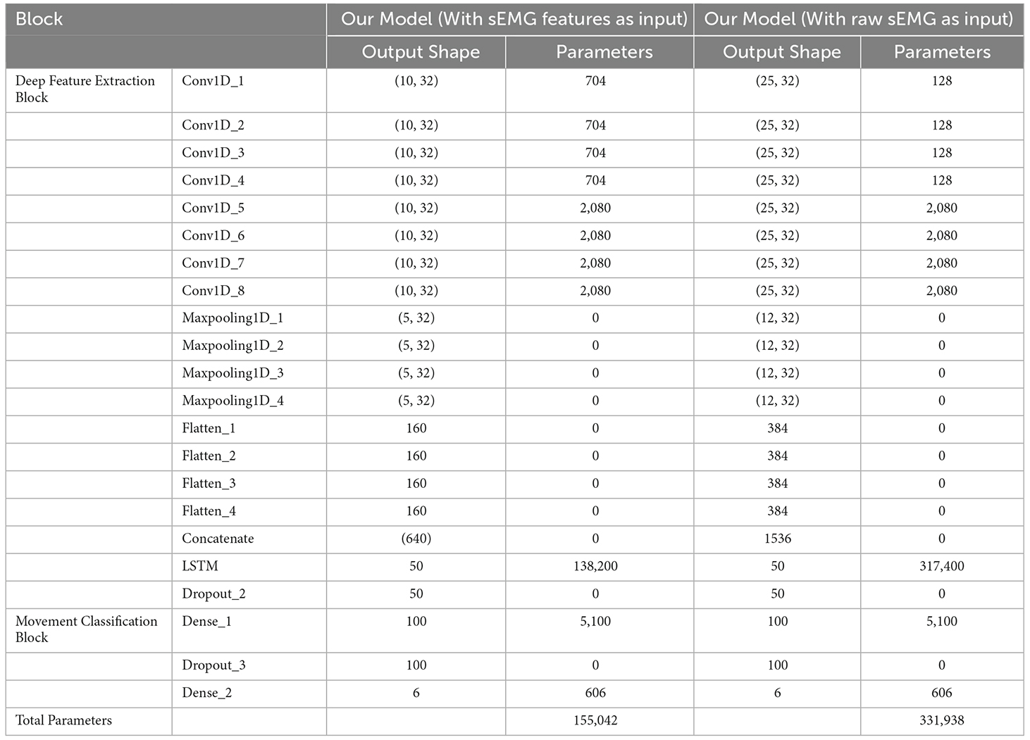
According to the relevant literature (Gautam et al., 2020; Bao et al., 2021), the batch size was set to be 256 and the number of epochs was set to be 100 in the training process. The specific parameters of the network model and the size of the deep learning feature vector of each layer are shown in Table 2. The model training and testing were performed on a PC that had AMD Ryzen 7 5800H CPU with 3.20 GHz, 16 GB RAM, and an NVDIA GeForce RTX 3050 Ti graphics card with 4 GB memory.

Table 2. Our model parameters details.

3. Experiment and results 3.1. Experimental protocol

Six male able-bodied subjects (age: 22–25 years old; height: 170–179 cm; weight: 60–75 kg) participated in this study. The subjects were asked to sit in a chair with their shanks dropping naturally and their whole body relaxed. This study was reviewed and approved by the Institutional Review Board of Xi’an Jiaotong University (Approval No. 2019-584).

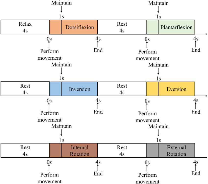
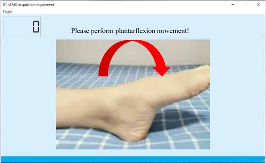
During the experiment, the subjects were asked to place their “unaffected side foot” (left foot) on the moving platform. The experimental procedure is shown in Figure 6. At the beginning of the experiment, the subjects were asked to relax and stare at a screen. A NeuSen WM (Neuracle Co., Ltd., China) was used as the sEMG acquisition equipment. The sampling frequency was 1,000 Hz, and the EMG electrodes were Ag/Cl electrodes. Before the experiment, the skin surface was wiped with alcohol to remove stains from the skin surface so as to reduce the impedance between the electrodes and the skin. After the experiments began, the subjects were asked to perform the movements to the maximum range shown on the screen. The specific process was as follows: (a) remaining relaxed for 4 s; (b) performing the ankle joint motion shown on the screen with a rotational speed as constant as possible until the rotation limit was reached, and this process should be finished within 1 s; (c) maintaining the rotational angle for 3 s; and (d) resting for 4 s and starting the next motion. A set of experiments contained six ankle movements. The subjects had a 5-min break between each two sets of experiments to prevent muscle fatigue. The screenshot of the guidance interface of the experiment is shown in Figure 7. Each subject was asked to repeat the experiment 12 times under each load. In total, 216 (3 loads × 6 movements × 12 times) trials of experiments were completed by each subject. As a result, 6 × 216 = 1,296 trials were completed. All participants were trained to do the isokinetic contraction by watching an animation of a 1-s constant rotation of the ankle joint on the computer monitor before the experiment to improve the consistency of the ankle rotation speed during the experiment. At the same time, the subjects moved their ankles along with the animation. During the experiment, the same animation also appeared on the computer monitor to help the subjects move at a constant speed.

Figure 6. Experimental procedure.

Figure 7. Screenshot of the guidance interface of the experiment.

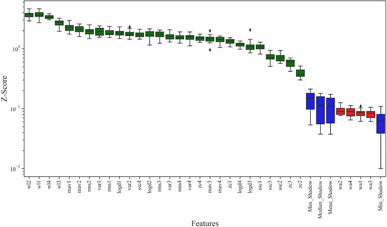
The result of the Boruta algorithm is shown in Figure 8. The feature marked in blue is the shadow feature represented by Max_Shadow, Median_Shadow, Mean_Shadow, and Min_Shadow. The Z-Score of Max_Shadow was recorded as Zmax, which was the criterion for judging the importance of features. Based on the Z-Score results, the feature suggested to be excluded was marked in red and seven features more related to ankle joint movements were marked in green. Therefore, seven features, including RMS, MAV, WL, ZC, SSC, VAR, and LogD, were selected to form the feature vector. In contrast, WA was not correlated with ankle joint movements and was excluded. Therefore, the number of selected features using the Boruta algorithm was 7.

Figure 8. Result of the Boruta algorithm: Z-Score was used to represent the feature importance. The features suggested to be excluded are marked in red, features more related to the dependent variables are marked in green, and the shadow features are marked in blue.

Therefore, according to the division of the window, a small window of 20 ms could achieve a feature vector with a size of 7 × 4. Also, a large window of 210 ms could obtain a feature matrix with a size of 20 × 7 × 4. Since the time step of LSTM was 2, the input size of the CNN-LSTM model was 10 × 7 × 4. We evaluated the performance of several models (CNN-LSTM, CNN, and LSTM) commonly used in sEMG recognition, with the raw sEMG and the features of sEMG as the inputs, to demonstrate the superiority of our model and the superiority of using the features of sEMG as the input (Atzori et al., 2016; Gautam et al., 2020; Ma et al., 2020).

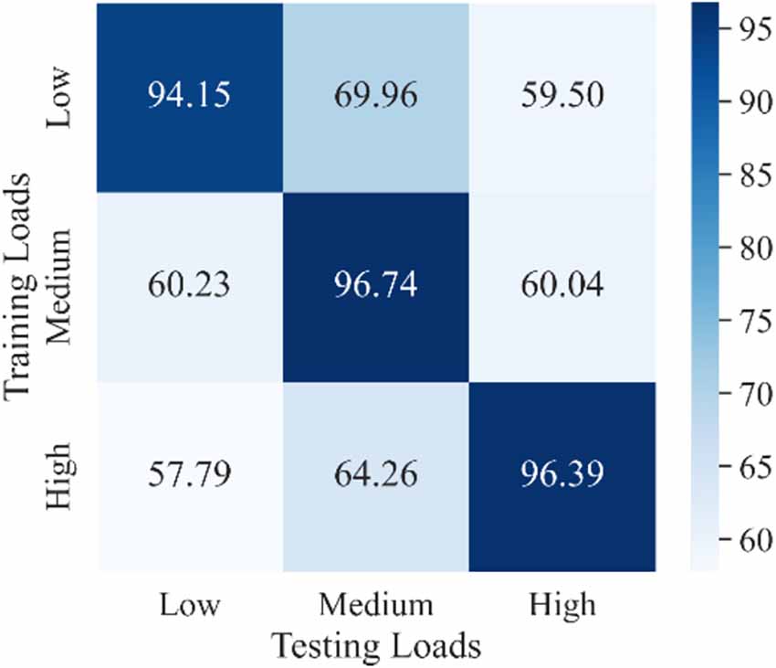
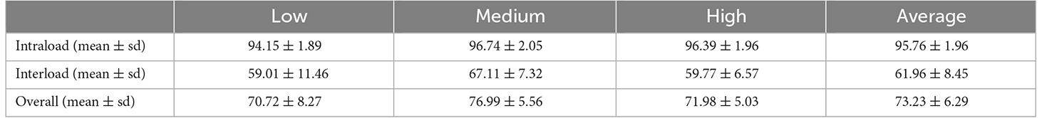
3.2. Experimental results 3.2.1. Effect of load variation on the accuracy of movement classification

As mentioned in the Introduction section, the load variation has a great influence on the classification accuracy in motion recognition using sEMG signals (Al-Timemy et al., 2013; Tang et al., 2016). However, most recent studies did not take the load variation into account when they trained their movement classification model. In other words, their models were trained without distinguishing the load levels, which was referred in this study as a one-step method. The purpose of the experiment discussed in this section was to demonstrate the effect of load variation on the accuracy of movement classification and provide a comparison object for our proposed two-step method discussed in the next section. Three CNN-LSTM models with the same architecture were trained under each load and then tested using data from all three loads. The classification results for all subjects represented using a confusion matrix are shown in Figure 9. The horizontal coordinate of the confusion matrix represents the load of the testing set, and the vertical coordinate represents the load of the training set. Each element in the confusion matrix represents the accuracy (in percentage) of all subjects for corresponding training and testing loads. Among these, the main diagonal elements represent the accuracy values in percentage where loads of the training and testing sets are the same [intraload (Tang et al., 2016)], and the off-diagonal elements represent the accuracy values in percentage where loads of the training and testing sets are different [interload (Tang et al., 2016)]. For example, 94.15 shows that the accuracy of classifying ankle movements under the low load by the trained CNN-LSTM classifier under the low load was 94.15%. Further, 69.96 represents that the accuracy of classifying ankle movements under the medium load by the trained CNN-LSTM classifier under the low load was 69.96%. Also, 60.23 represents that the accuracy of classifying ankle movements under the low load by the trained CNN-LSTM classifier under the medium load was 60.23%. The average value and variance of accuracy under intraload, interload, and all loads are shown in Table 3. The overall accuracy in Table 3 represents the average accuracy of all subjects under intraload and interload when using the one-step method. The two-sample t-test was then conducted. Based on the test result (data were normal distribution using the Shapiro-Wilk test, P = 1.34E-18 < 0.001), it was suggested that a significant difference existed in the accuracy between intraload and interload. It indicated that the load variation had a substantial influence on the accuracy of movement classification. This revealed that the robustness of the one-step method was not good enough regarding the load variation.

Figure 9. Confusion matrix of classification results for all subjects under every single load using a one-step method. Each element represents the accuracy of all subjects for corresponding training and testing loads. Darker color indicates higher accuracy. The main diagonal elements represent the accuracies where the load of training and testing sets are the same. The off-diagonal elements represent the accuracies where the load of training and the testing sets are different.

Table 3. Average value and variance of accuracy under intraload, interload, and all loads using a one-step method.

3.2.2. Comparison between the proposed two-step method and other conventional methods

In this study, we proposed a two-step method with a CNN-LSTM model to classify ankle movements. The first step was to calculate the RMS of sEMG and feed it into the Random Forest classifier for load classification. The Random Forest classifier was selected to recognize a specific load in this article because of its remarkable robustness and good resistance to overfitting (Zhou et al., 2019). Each subject performed six movements under a single load. Each movement was performed 12 times and lasted for 4 s. In order to reduce the influence of the movement process on the sEMG signals, 200 ms signals before and after each movement were removed. Therefore, each movement lasted for 3.6 s. The total length of sEMG signals recorded for each subject was 6 × 12 × 3.6 = 259.2 s. The number of samples per subject under a single load can be then calculated using equation (3).

Ns=T−window lengthsliding length(3)

where Ns is the number of samples per subject under a single load, and T is the effective time of sEMG signals from each subject under a single load. Since the sliding length was 120 ms and the window length was 210 ms, the number of samples per subject under a single load was calculated to be 2,158.

Therefore, the number of samples per subject under all loads was 6,474. Since these samples were randomly divided into a training set and a testing set using a ratio of 8:2, the number of training and testing samples per subject under all loads was 5,179 and 1,295, respectively. Therefore, the number of training and testing samples for six subjects under three loads was 5,179 × 6, and 1,295 × 6, respectively. The total number of samples was 38,844, comprising six subjects under three load levels. In the training phase, a five-fold cross-validation strategy (where four-folds were used for training and one-fold was used for validation) was used to improve the consistency of the classification results. As a result, the number of samples for the training set under the low load recognized by the Random Forest classifier was 10,325 and the number of samples for the testing set was 2,623. The number of samples for the training set under the medium load recognized by the Random Forest classifier was 10,375, and the number of samples for the testing set was 2,573. The number of samples for the training set under the high load recognized by the Random Forest classifier was 10,374, and the number of samples for the testing set was 2,574. The training and testing sets were not of exactly the same size under each load level because of the randomness when dividing the datasets.

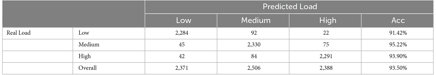
The classification results of the Random Forest classifier were then obtained (Table 4). The data in Table 4 represent the number of samples predicted to the corresponding load of the column. The average accuracy of the Random Forest classifier for all three loads was 92.81%, which could fulfill our requirements. In the second step, according to the identified load category, the features of sEMG were sent to the trained CNN-LSTM model with the same load category for movement classification.

Table 4. Results of load classification.

The results of movement classification are shown in Table 5. The first three columns of data in Table 5 show the number of samples in the classified load category that the movements are correctly identified, and the last column is the accuracy of movement classification. Using Table 3 as a reference, we could clearly see the advantages of the two-step method. The accuracy under low, medium, and high loads increased from 70.72%, 76.99%, and 71.98% to 91.42%, 95.22%, and 93.90%, respectively. The overall accuracy of movement classification increased from 73.23% to 93.50%. In addition, a two-sample t-test was conducted. The P-value of overall accuracy between the two-step and conventional methods was 7.90E-4. It was suggested that a significant difference existed in the accuracy between these two methods. Therefore, it was concluded that the proposed two-step method could greatly improve the accuracy of classification compared with the conventional one-step method.

Table 5. Results of movement classification using our proposed two-step method.

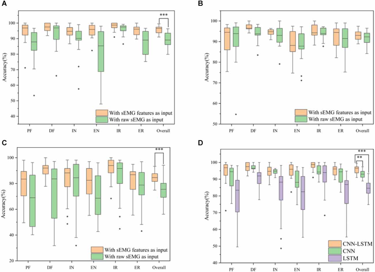
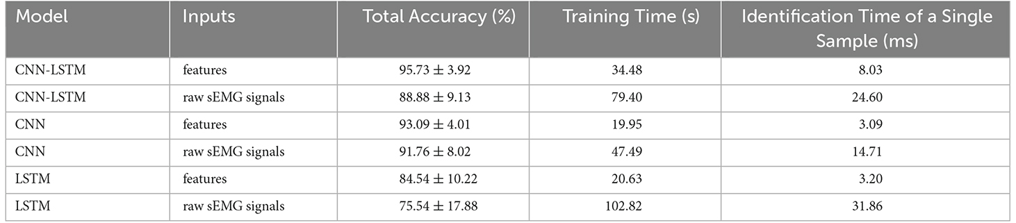
3.2.3. Comparison among different models

Several model architectures with the sEMG features and the raw sEMG as inputs were compared to verify the performance of the proposed CNN-LSTM model with sEMG features as the input, as shown in Figure 10. It was obvious that the accuracy with sEMG features as the input was higher than that with raw sEMG as the input when using the CNN-LSTM, CNN, and LSTM models. The accuracy of the CNN-LSTM, CNN, and LSTM models with sEMG features as the input was 6.85%, 1.33%, and 9.00% higher than that of the corresponding models with raw sEMG as the input, respectively. A statistical analysis was conducted to explore the influence of different inputs on accuracy. According to the two-sample t-test (data were normal distribution using the Shapiro-Wilk test), the P-value of the CNN-LSTM, CNN, and LSTM models was 1.16E-05, 0.17, and 8.50E-04, respectively. It was suggested that a significant difference existed in the accuracy between sEMG features and raw sEMG as the inputs when using the CNN-LSTM and LSTM models. Meanwhile, we removed the Boruta algorithm and tested the CNN–LSTM model using all eight time-domain features to verify the significant improvement using the Boruta algorithm. The results showed that the classification accuracy of the CNN-LSTM model decreased from 95.73% to 92.84% after the Boruta algorithm was removed. A two-sample t-test (P = 0.004 < 0.01) was conducted, which showed that the performance of the model significantly improved when using the Boruta algorithm. In addition, the parameters of the CNN-LSTM model with sEMG features as the input was 155,042, while the parameters of the CNN-LSTM model with raw sEMG as the input was 331,938. Therefore, the computation cost of our method was only 46.70% of that of the conventional method. In addition, we calculated the time required to train these three models with sEMG features and with sEMG as the inputs. The total time required for each model with sEMG features as the input was equal to the time required for feature extraction plus the time required for training. The total time required by the CNN-LSTM, CNN, and LSTM models with sEMG features as the input was 34.48 s, 19.95 s, and 20.63 s, which was 44.92 s, 27.54 s, and 82.192 s less than that of the corresponding models with raw sEMG as the input, respectively. Moreover, the identification time of a single sample was calculated. The average identification time of a single sample required by the CNN-LSTM, CNN, and LSTM models with sEMG features as the input was 8.03 ms, 3.09 ms, and 3.20 ms, which was 16.57 ms, 11.62 ms, and 28.66 ms less than that of the corresponding models with raw sEMG as the input, respectively, guaranteeing the real-time control of rehabilitation robots.

Figure 10. Classification accuracy for six movements using different models. (A) CNN-LSTM model with sEMG features and raw sEMG as the inputs. (B) CNN model with sEMG features and raw sEMG as the inputs. (C) LSTM model with sEMG features and raw sEMG as the inputs. (D) Classification accuracy for six movements using different network architectures with feature extraction (*P-value < 0.05, **P-value < 0.01, and ***P-value < 0.001).

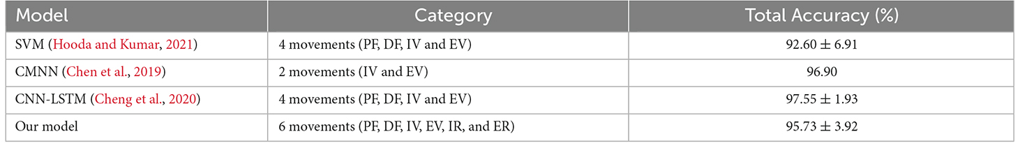
Our model was compared with CNN, LSTM, SVM models used in the study by Hooda and Kumar (2021), the CNN-LSTM model used in the study by Cheng et al. (2020), and the CMNN model used in the study by Chen et al. (2019) to verify the superior performance of the proposed model. Figure 10D, Tables 6 and 7 show the results of the aforementioned evaluation. It is worth mentioning that the results of the CNN model, LSTM model, and our proposed model were from the classification performance with the same dataset collected in the present study, whereas the results of the SVM (Hooda and Kumar, 2021), CNN-LSTM (Cheng et al., 2020), and CMNN (Chen et al., 2019) models were from the reported conclusions in the existing studies (Chen et al., 2019; Cheng et al., 2020; Hooda and Kumar, 2021). The accuracy of the CNN-LSTM model was 2.64% and 11.19% higher than that of the CNN and LSTM models, respectively. A two-sample t-test was conducted. According to the test result (data were normal distribution using the Shapiro-Wilk test), the P-value between the CNN-LSTM and CNN models was 0.002 (less than 0.01), and the P-value between the CNN-LSTM and LSTM models was 5.07E-10 (less than 0.001). It was suggested that a significant difference existed in the accuracy between the CNN-LSTM, CNN, and LSTM models. It indicated that the CNN-LSTM model had significant superiority over the CNN and LSTM models. Compared with the SVM classifier proposed by Hooda and Kumar (2021) the accuracy of the CNN-LSTM model was 3.13% higher. Moreover, the CNN-LSTM model proposed in this article could classify six movements including PF, DF, IV, EV, IR, and ER, whereas the SVM classifier proposed by Hooda and Kumar (2021) could only classify four movements, namely PF, DF, IV, and EV. Compared with the CMNN classifier proposed by Chen et al. (2019) and the CNN-LSTM hybrid model proposed by Cheng et al. (2020), the accuracy of the CNN-LSTM model was 1.17% and 1.82% lower, respectively. However, the CMNN model can only classify two movements, including IV and EV, and the model proposed by Cheng et al. (2020) can only classify four movements, including PF, DF, IV, and EV. In addition, the raw sEMG instead of features was fed into the model proposed by Cheng et al. (2020), which involved huge computational costs.

Table 6. Performance of different network architecture and inputs.

Table 7. Comparison with the state-of-the-art method.

Please note that the differences between the proposed CNN-LSTM and the CNN-LSTM proposed by Cheng et al. (2020) are as follows. (1) The input processes for those two models were different. In our proposed CNN-LSTM, the sEMG signals collected from four channels were fed into CNN respectively. They were flattened and concatenated after convolution. In the CNN-LSTM proposed by Cheng et al. (2020), the sEMG signals of all channels were fed together for convolution. (2) The outputs of these two modes were different. The output of our model was six categories, while that of the CNN-LSTM proposed by Chen et al. (2020) was four categories; and (3) The convolution layer, LSTM layer, and Dense layer of these two models had different number of layers and parameters.

4. Discussion 4.1. Classified ankle movements

As mentioned earlier, the current literature mainly focused on gait recognition rather than on ankle movement classification for lower-limb rehabilitation training (Varol et al., 2010; Joshi et al., 2013; Gautam et al., 2020). The reason might be that the ankle joint could perform six movements, and it is more difficult to accurately decode those six movements than gait recognition using sEMG signals. Two ankle movements including IV and EV could be classified with an accuracy of 96.90% by the method proposed by Chen et al. (2019). The models proposed in the studies by Hooda and Kumar (2021) and Cheng et al. (2020) could classify four ankle movements (PF, DF, IV, and EV) with an accuracy of 92.60% and 97.55%, respectively. IR and ER movements could be recognized incorrectly because the PF/DF of the ankle was always accompanied by IR/ER (Chen, 2018). Whether applying the methods used in these previous studies could classify these six movements and maintain high accuracy remains to be explored.

In this study, our model can classify six ankle movements with an accuracy of 95.70%. Compared with the models in the aforementioned studies, our model can classify more ankle movements with relatively good accuracy. Our target is to use the decoded movements of the unaffected side to control the robot-assisted motion on the affected side of stroke patients.

4.2. Feature extraction

The timing of paired human movement intent and associated feedback is critical to induce neuroplasticity (estimated to be within 300 ms) during rehabilitation training (Hudgins et al., 1993). Therefore, reducing decoding time movement intent from sEMG is an important task. Deep learning models such as CNN can be used as classifiers to classify ankle movements. However, normally raw sEMG signals are directly fed into the model, which brings heavy calculation burden; thus, the real-time performance cannot be guaranteed. In our study, seven time-domain features were selected using the Boruta algorithm. Then, these features were fed into our CNN-LSTM model. To our best knowledge, this is the first time that the Boruta algorithm is used for feature selection of sEMG, and it is also the first time that selected features rather than raw sEMG are fed into a CNN-LSTM model. In addition, adding more layers to the network might improve the accuracy. However, the computational cost will increase, which will affect the real-time performance. The aim of selecting time-domain features with the Boruta algorithm and feeding them into the network is to find a balance, which can not only obtain high accuracy but also meet the requirements of real-time performance.

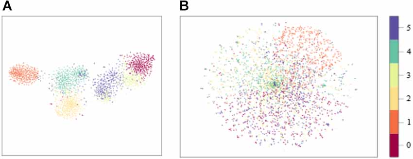
The distribution of model input with sEMG features and raw sEMG is visualized in Figure 11 with t-Distributed Stochastic Neighbor Embedding (t-SNE), where the dimension of model input was reduced from high dimension to 2D. We could see that the boundaries of each class with sEMG features as the input were clearer than those with raw sEMG as the input. As a result, the convergence speed of the model with sEMG features as the input would be larger. The time required to train these three models with sEMG features and raw sEMG as the inputs was calculated. The total time required by these three models with sEMG features as the input is all less than that of the corresponding models with raw sEMG as the input. Also, the time required by the CNN-LSTM model was longer than that required by the CNN and LSTM models. This might be because the CNN-LSTM model is more complex and has more parameters. In the future study, we should find ways to reduce the parameters of the CNN-LSTM model and the training time while maintaining high accuracy. On the contrary, using our proposed CNN-LSTM model, the ankle movement classification time of a single sample was only 8.03 ms, which was about 5 ms longer than that using the CNN or LSTM model. It would not be difficult to meet the real-time requirement (300 ms) of rehabilitation even considering other time delay factors in the rehabilitation system (Hudgins et al., 1993). As shown in Table 6; the average accuracy of the CNN-LSTM, CNN, and LSTM models with features of sEMG as the inputs was higher than that with the raw sEMG signals as the input. In addition, the statistical analysis results showed that the input of the CNN-LSTM and LSTM models had a significant impact on the accuracy whereas no significant difference on accuracy was found between the CNN-LSTM and CNN models. This might be because the CNN model has a good deep feature extraction performance. In the future study, the specific reason should be found.

Figure 11. Distribution of features. (A) CNN-LSTM model input with sEMG features as the input. (B) CNN-LSTM model input with raw sEMG as the input.

4.3. Load variation

Different load levels will lead to different levels of muscle activity, and sEMG reflects the level of muscle activity (Kiguchi and Hayashi, 2012). If the classifier trained under a single load is used to classify the sEMG signals under other loads, the accuracy will be greatly reduced (33.80%), as shown in Table 3. Tang et al. (2016) found that putting EMG signals under all loads together into the model could not achieve an ideal performance when decoding the elbow joint angle. In this study, we used a two-step method to reduce the effect of load variation on the classification results of ankle movements. In the proposed two-step method, multiple CNN-LSTM models were trained under different loads. In this study, we trained three CNN-LSTM models under three loads (low, medium, and high). When adopting the two-step method, a random forest classifier was used to classify the load first, and then the corresponding CNN-LSTM model was selected to classify the movement. As shown in Tables 3 and 5, the overall accuracy improved from 73.23% to 93.50% using the two-step method. Unfortunately, errors existed (7.19%) when using the Random Forest classifier to classify the load. In other words, some signals of a specific load were fed into trained models under a different load level which it should not belong to. In future studies, improving the accuracy of load level recognition is the direction of our efforts. In addition, we only used three load levels (low, medium, and high) in this study. However, in practical applications, the load may not be within the training range. Expanding the training pool and dividing the load levels more finely may be a solution. Another factor that has a certain impact on accuracy is fatigue (Enoka et al., 2011). In this study, the problem was addressed by giving the subjects plenty of time to rest during the experiment. Our data were not collected under fatigue. In future studies, fatigue should also be taken into account.

4.4. Different models

In this study, we adopted the CNN-LSTM model to classify ankle movements. The model consisted of two convolution layers, one LSTM layer, and two dense layers. The hyperparameters of our model were mainly determined with reference to previous studies and then manually tuned via experience (Gautam et al., 2020). We compared the performance of our model with that of other models and performed the statistical analysis. As shown in Table 6, the accuracy of our CNN-LSTM model was higher than that of the CNN and LSTM models. The statistical analysis results indicated that the CNN-LSTM model had significant superiority over CNN and LSTM models. Furthermore, the validation of our model for ankle movements classification is shown in Table 7 along with a comparison with the CMNN (Chen et al., 2019), CNN-LSTM (Cheng et al., 2020), and SVM (Hooda and Kumar, 2021) state-of-the-art models. Unfortunately, since not many researchers focused on classifying the ankle movements alone using sEMG signals, finding any suitable public datasets to further verify the robustness of our method was difficult. Please note that, since detailed information about the computational costs of these three models [SVM (Hooda and Kumar, 2021), CNN-LSTM (Cheng et al., 2020), and CMNN (Chen et al., 2019) models] was not found, only the classification accuracy was compared between these three models and our proposed CNN-LSTM model. Further investigation regarding the computation complexity or computation efficiency of those models are desired in the future study.

As mentioned in Section “2.4 Network architecture”, after the pre-processing, a feature matrix with the size of 20 × N was obtained for each channel (four channels in total). The feature matrix used in our proposed CNN–LSTM model, the conventional CNN, and LSTM models was the same. However, the input dimensions to these models were different because the requirements of these three models were different. The input dimension of CNN was 20 × N. The input of the traditional LSTM model is required to be a one-dimensional vector. Therefore, in this study, the feature matrix was flattened to become a one-dimensional input vector before being fed into the LSTM model. The input dimension for the proposed CNN-LSTM model is related to the time step. Because the time step was set to 2, the 20 × N feature matrix was divided into two 10 × N input matrices before being fed into the CNN-LSTM model. Each 10 × N matrix was used as the input for each step. Although the dimensions were different, the feature matrix used in these three models was the same. Therefore, in this study, we considered that the fairness of comparison could be guaranteed. In future studies, the influence of the input dimensions should be investigated in detail. Another possible direction is to find a way to keep the input dimension the same when using different models.

4.5. Limitations and future directions

This study had a few limitations. First, in our study, all the subjects were healthy male subjects and the number of subjects was not large enough. The age of the subjects was 22–25 years. In future studies, the diversity of the subjects should be increased. Moreover, the sEMG signals on the unaffected side of stroke patients may be different from those of healthy people. Hence, in future studies, the validation experiments should involve stroke patients.

The second limitation was the classification speed. Although we adopted some methods such as feature extraction to improve the classification speed, using the CNN-LSTM model still required more parameters. Most of the parameters were in the LSTM layer. However, the LSTM layer was critical in our model, which was used to extract the correlation on the time sequence. Therefore, in future studies, we should try to reduce the parameters of the LSTM layer while ensuring accuracy.

In this study, we proposed a CNN-LSTM model for the first time to classify ankle movement using sEMG signals. Compared with the previous methods (Varol et al., 2010; Joshi et al., 2013; Gautam et al., 2020), the performance of our method has been already greatly improved. As we all know, deep learning develops rapidly. In the last few years, some novel models have been developed and used to classify the movements of the hand and wrist joints, for example, CNN-BiLSTM (Nguyen-Trong et al., 2021; Tripathi et al., 2022) and Graph Convolutional Network (GCN; Lai et al., 2021; Yang et al., 2022). However, to the best of our knowledge, they have not been used in studies to classify ankle movements. In future studies, we will adopt these novel models and compare them with our proposed ones.

The method we proposed in this study could accurately classify these six ankle movements using sEMG signals. As we all know, the movement of the human wrist is quite similar to that of the ankle joint. Therefore, we can try to apply our method to the decoding of human wrist movements in the future.

In this study, we provided the basis of the ankle movement classification for robot-assisted bilateral rehabilitation training. Although some researchers have realized robot-assisted bilateral rehabilitation training for patients based on sEMG signals for other parts of the body, for example, the hands (Leonardis et al., 2015), this concept has not been applied to ankle rehabilitation. Realizing the concept of using the unaffected side for the robot-assisted motion control on the affected side in ankle rehabilitation may be challenging due to the different motion patterns or constraints between the intact side and the affected side for stroke survivors. These should be explored in future studies.

5. Conclusion

In this article, a time-domain feature selection method of the sEMG, a CNN-LSTM model, and a two-step method were proposed to decode the movement intention of the ankle joint for bilateral ankle rehabilitation training to classify more ankle movements, reduce the computational cost, and minimize the influence of load variation on classification results. For the first time, the Boruta algorithm was used in this study to select time-domain features of sEMG. The selected features rather than raw sEMG were fed into the CNN-LSTM model. Hence, the parameters of the model were reduced from 331,938–155,042. Experiments were conducted to verify the proposed method. The results showed that our method could classify six ankle movements with relatively good accuracy (95.70%). The total time required by the CNN-LSTM, CNN, and LSTM models with sEMG features as the input was all less than that of the corresponding models with raw sEMG as the input. In addition, the accuracy of the CNN-LSTM, CNN, and LSTM models with sEMG features as the input was all higher than that of the corresponding models with raw sEMG as the input. The overall accuracy was improved from 73.23% to 93.50% using our two-step method for classifying the ankle movements with different loads. Our proposed CNN-LSTM model had the highest accuracy in ankle movements classification compared with the CNN, LSTM, and SVM models.

Data availability statement

The datasets presented in this study can be found in online repositories. The names of the repository/repositories and accession number(s) can be found below: https://ieee-dataport.org/documents/semg-signals-ankle-movement-under-different-loads.

Ethics statement

The studies involving human participants were reviewed and approved by Institutional Review Board of Xi’an Jiaotong University. The patients/participants provided their written informed consent to participate in this study.

Author contributions

ML and JW: conceptualization and methodology, experiment design, data analysis. ML: supervision. JW and SY: investigation. ML, JW, JX, GX, and SL: writing. ML and SL: funding acquisition. All authors contributed to the article and approved the submitted version.

Funding

This work was supported in part by the National Natural Science Foundation of China under Grant (51975451) and the EPSRC project “ViTac: Visual-Tactile Synergy for Handling Flexible Materials” (EP/T033517/1).

Acknowledgments

We thank the participants and all those who provided help and advice in the experiment.

Conflict of interest

The authors declare that the research was conducted in the absence of any commercial or financial relationships that could be construed as a potential conflict of interest.

Publisher’s note

All claims expressed in this article are solely those of the authors and do not necessarily represent those of their affiliated organizations, or those of the publisher, the editors and the reviewers. Any product that may be evaluated in this article, or claim that may be made by its manufacturer, is not guaranteed or endorsed by the publisher.

References

Ahmadizadeh, C., Pousett, B., and Menon, C. (2019). Investigation of channel selection for gesture classification for prosthesis control using force myography: a case study. Front. Bioeng. Biotechnol. 7:331. doi: 10.3389/fbioe.2019.00331

PubMed Abstract | CrossRef Full Text | Google Scholar

Akbari, A., Haghverd, F., and Behbahani, S. (2021). Robotic Home-Based rehabilitation systems design: from a literature review to a conceptual framework for community-based remote therapy during COVID-19 pandemic. Front. Robot. AI 8:612331. doi: 10.3389/frobt.2021.612331

PubMed Abstract | CrossRef Full Text | Google Scholar

Al-Quraishi, M. S., Ishak, A. J., Ahmad, S. A., and Hasan, M. K. (2015). “Impact of feature extraction techniques on classification accuracy for EMG based ankle joint movements,” in Control Conference, (Kota Kinabalu, Malaysia: IEEE), 1–5.

Google Scholar

Al-Timemy, A. H., Bugmann, G., Escudero, J., and Outram, N. (2013). “A preliminary investigation of the effect of force variation for myoelectric control of hand prosthesis,” in Annual International Conference IEEE Engineering in Medicine and Biology Society, (Osaka, Japan: IEEE), 2013, 5758–5761.

Google Scholar

Al-Timemy, A. H., Khushaba, R. N., Bugmann, G., and Escudero, J. (2016). Improving the performance against force variation of EMG controlled multifunctional Upper-Limb prostheses for transradial amputees. IEEE Trans. Neural Syst. Rehabil. Eng. 24, 650–661. doi: 10.1109/TNSRE.2015.2445634

PubMed Abstract | CrossRef Full Text | Google Scholar

Ang, K. K., Guan, C., Phua, K. S., Wang, C., Zhou, L., Tang, K. Y., et al. (2014). Brain-computer interface-based robotic end effector system for wrist and hand rehabilitation: results of a three-armed randomized controlled trial for chronic stroke. Front. Neuroeng. 7:30. doi: 10.3389/fneng.2014.00030